Chapter 4 Installing and using packages (libraries)
R is open source which means that anyone can contribute to R by making packages. Packages or libraries are collections of R functions, data, and codes stored in a format. R and RStudio come with several standard packages, but there are also options to download packages made by other people. All packages made by other people are uploaded to http://cran.r-project.org and at the time of writing of this book, there are 16065 packages available for download. There are a lot of packages with all kinds of possibilities. For example, you can use the readxl package to load excel data and you can use the ggplot2 package to create beautiful visualizations.
Within this chapter, we will look at how to install and use the packages. Like most things, there are several options on how to do this. For now, we will explain 2 options to install packages or libraries.
- Option 1: Let RStudio install the packages
- Option 2: Installing the packages yourself
4.1 Option 1
To let RStudio install packages we can click on Tools at the top of RStudio and then click on Install Packages…. When we have clicked on this we will see the following screen:
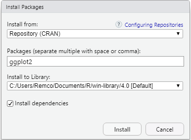
Figure 4.1: RStudio packages
In the top bar, we see that we are installing the packages from CRAN and you can leave this as is (the other option is to download the packages directly to your computer from CRAN and install them using a zip file). Furthermore, we can type in the 2nd bar which packages we want to install. As an example, we will install the ggplot2 package here. Further on in this book, we will use some packages that are not installed automatically, but that will be indicated when necessary.
In the 3rd and last bar, you will find where the packages will be installed and you don’t need to change this because R will automatically create a folder for downloaded packages. Finally, we see an option to install dependencies and you should always check this option.
If you download a package and that package needs other packages to work properly or perform certain functions, these will be downloaded automatically when you check the option to install dependencies.
We can also install multiple packages at the same time in this screen by typing multiple packages in the 2nd bar and placing a space or comma between the packages. Below we see an example where we install both the ggplot2 and the readxl package.
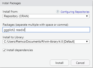
Figure 4.2: Installing multiple packages
If everything is ok then we can press Install. Afterward, the packages will be installed and you will see something similar to the screen below:
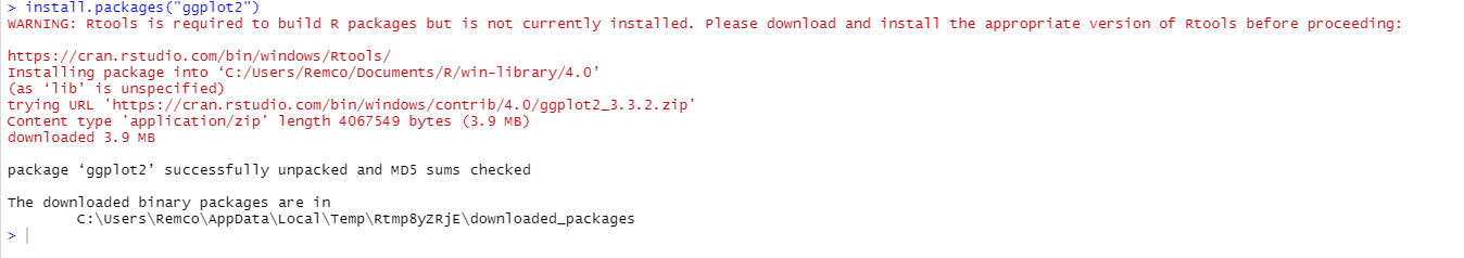
Figure 4.3: Installation console
We can see in red that RStudio downloads the package from Cran and in black we see that the package ggplot2 is installed and in which location it is installed.
4.2 Option 2
There is also a second option to install packages and that is to type in the code yourself. If we look at the last picture of option 1, we see in blue that the following code is executed: install.packages (“ggplot2”). Of course, we can also type this code ourselves in a new file. If we want to download the ggplot2 package again we can type the following code in a new file:
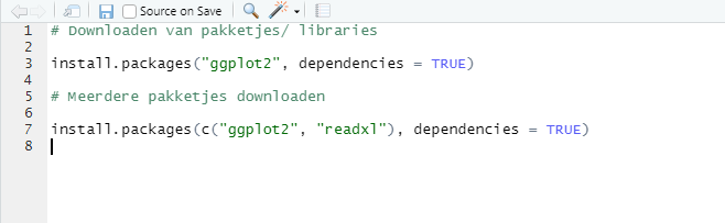
Figure 4.4: Installing packages
install.packages("ggplot2", dependencies = TRUE)Within this code we also see dependencies = TRUE, this indicates that it must also install all dependencies of the package you want to install (just like how we installed dependencies for option 1). To install multiple packages at the same time we can again use the c function to specify multiple things at the same time. So if we want to install the readxl packet together with the ggplot2 packet just like in option 1, we can do that by typing the following code in a file and then selecting and running the code as explained in the previous chapter.
install.packages(c("ggplot2", "readxl"), dependencies = TRUE)Choose whatever option that seems easier to install packages and then we will proceed to update packages.
4.3 Updating packages/ libraries
There are also 2 options to update packages. We can either type the code ourselves or we can use RStudio to update our packages.
Let’s start by typing the code ourselves to update packages. This is simply done by using the update.packages() function. If you want to update all packages simply type in a new file or in the console:
update.packages()Next, for each package, you want to update you will get a pop-up where you can choose whether or not you want to update the packages.
Suppose you only want to update a specific package, for example, the ggplot2 package you type the following:
update.packages("ggplot2")We can also let RStudio update our packages. In the box on the bottom-right of RStudio, we have next to the Files and Plots options also an option named Packages. When we click on this option we see many packages and we also see a green button update. When we click on this update button we get a list of packages that have a newer version. You can choose to update individual packages by checking the box on the left side or you can update them all at once by pressing select all and then press Install updates.
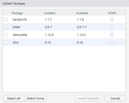
Figure 4.5: Updating packages
4.4 Using packages
Now that we know how to install and update packages we reach the last step and that is to use packages. As already mentioned, we can use the readxl packet to open excel files. First, we will look at what happens when we try to use the functions of a package that we have installed but haven’t loaded yet.
For example, if we want to use the function read_excel() from the readxl package to open an excel file we type the following code:
read_excel("excelbestand.xlsx")Afterward, we see a red warning that says: Error … could not find function “read_excel”.
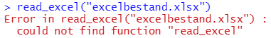
Figure 4.6: Erro could not find function
Usually, that means one of 2 things: - We wrote the function wrong - Or we wrote the function correctly but we didn’t load the package of that function.
In this case, it is the 2nd option. If we want to use the functions of packages we always need to load the specific package. We can do that with the following code:
library(readxl)And now we can use the read_excel function.
This was a small example of how we can open files and in this case, the data consists of 2 columns with only 8 data points. Later on, we will look in more detail at how we can load data and what exactly we can do with it.
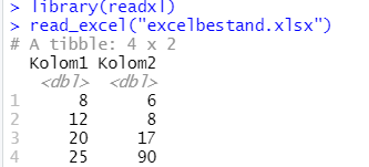
Figure 4.7: Loading a library
4.5 Tidyverse
Tidyverse is a collection of libraries specifically designed for data manipulation, data exploration, and data visualization. If you have installed the tidyverse library and subsequently load it, R will automatically load the following libraries:
- ggplot2
- dplyr
- tidyr
- readr
- tibble
- stringr
- forcats
- purr
These are all commonly used libraries that can be used for different purposes. Often things can be accomplished in different ways and certain solutions from the tidyverse library are easier, better readable, or simply better. For example, with the ggplot2 library, you have a lot more options to customize visualizations, you can choose from more types of visualizations, and the visualizations almost always look better than the visualizations that can be made with other libraries.
Within this book, we can not discuss all these libraries, but we will explain the ggplot2 library later on. Besides that, we will discuss some functions and look at the tidyverse equivalent. Finally, we will look at the “pipe” operator which is written as follows: %>%. This pipe operator is part of the magrittr library, but will also be available when we have either loaded the dplyr or tidyverse libraries.
For now, we will load the library dplyr to show the usage of this pipe operator.
library(dplyr)The pipe operator %>% is written as a percentage sign, followed by an arrow to the right and then another percentage sign. This pipe operator is often found in other’s codes and to show what it does and why it is useful we will take a look at the following example:
If we have multiple numbers in a vector, for example, 1, 8, 9, 14, and 18 and we want to take the square root of these numbers and then get the average, we can do it as follows without the pipe operator:
mean(sqrt(c(1, 8, 9, 14, 18)))## [1] 2.962545We use 3 functions here namely, mean() to get the average, sqrt() to take the square root, and the c() function to make a vector with multiple numbers.
It is possible in R to use multiple functions in one line of code and one thing to notice is that this code has to be interpreted from the inside out. You can imagine that if we want to use more functions it will be difficult to read.
The pipe operator offers an elegant solution here and what it does is to take the previous argument onto the next one. So the following code is the same as the example above:
c(1, 8, 9, 14, 18) %>%
  sqrt() %>%
  mean()
## [1] 2.962545This time you can read the code from left to right instead of inside out. It takes the numbers, takes their square roots, and then takes the average of all these numbers.
This pipe operator can be used consecutively on a line, but you can also separate multiple functions on a new line. As long as the pipe operator is used at the end of a line this works as well:
c(1, 8, 9, 14, 18) %>%
sqrt() %>%
mean()## [1] 2.962545