Chapter 10 Glm function for regression
We can use the glm() function in R to perform different regression types. Within this book, we will discuss linear regression and logistic regression, and we will briefly discuss other options that we can use by using the glm() function.
10.1 Linear regression
We will start by looking at linear regression. Linear regression is used for 2 purposes, namely for association or prediction. Within this chapter, we will mainly look at association, in other words, to see if there is a relationship between two variables. To explain this, we will look at an example with systolic blood pressure and age.
First, we will have to load some data, and in this case, it is an SPSS file called sbp_age. To load this, we use the foreign() package we have seen before.
library(foreign)
sys_bloodpressure <- read.spss("sbp_age.sav", to.data.frame = TRUE)
## re-encoding from UTF-8The data is stored in the variable called sys_bloodpressure, and we can look at the first observations by using the head() function again.
head(sys_bloodpressure)## pat_id sbp age
## 1 1 144 39
## 2 2 220 47
## 3 3 138 45
## 4 4 145 47
## 5 5 162 65
## 6 6 142 46We see that this dataset has three variables, namely pat_id, sbp for the systolic blood pressure, and age. We can visualize the association/relationship between systolic blood pressure and age by using a scatterplot (again, we will discuss visualizations in further depth in the visualization chapter).
plot(sys_bloodpressure$age, sys_bloodpressure$sbp)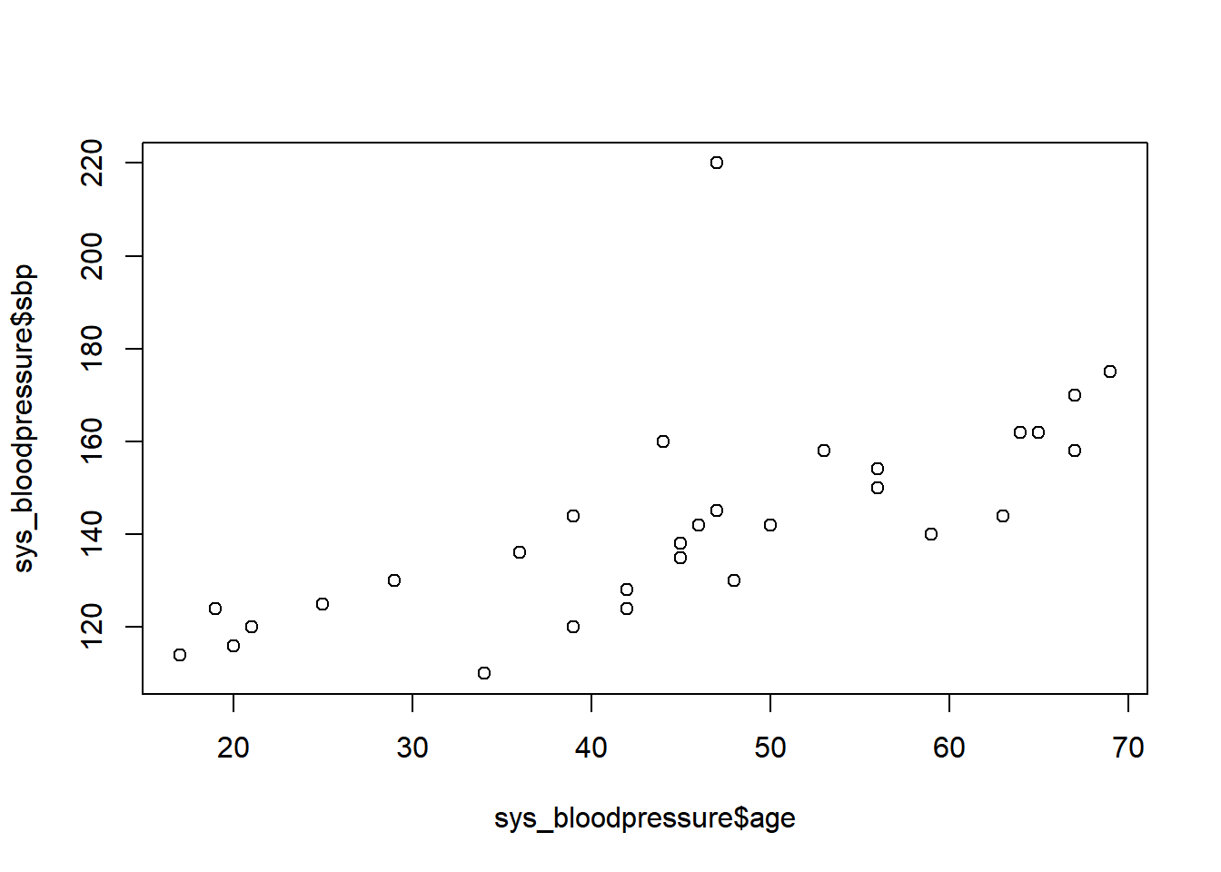
You may have already noticed when we looked at the first observations that there was a patient with a systolic blood pressure of 220. In the scatterplot, we can see that this value is very different from the other observations. Therefore, this is called an outlier. Normally, we have to be careful with outliers, and we have to be sure whether or not this value is plausible, and whether or not we should keep it in the data. For now, we are going to remove this value and make this value missing.
If we only want to remove that specific value of systolic blood pressure, then we can look at what observation it was. In this case, we already know that the second patient had a systolic pressure of 220. We can check this again by indexing the systolic blood pressure of the second patient.
sys_bloodpressure$sbp[2]## [1] 220Here we see that the systolic blood pressure of the second patient was indeed 220. If we want to make this value missing, we can simply overwrite this value with NA for missing. We can do that as follows:
sys_bloodpressure$sbp[2] <- NAand now we have made this value missing.
If we look at the scatterplot again with the same code:
plot(sys_bloodpressure$age, sys_bloodpressure$sbp)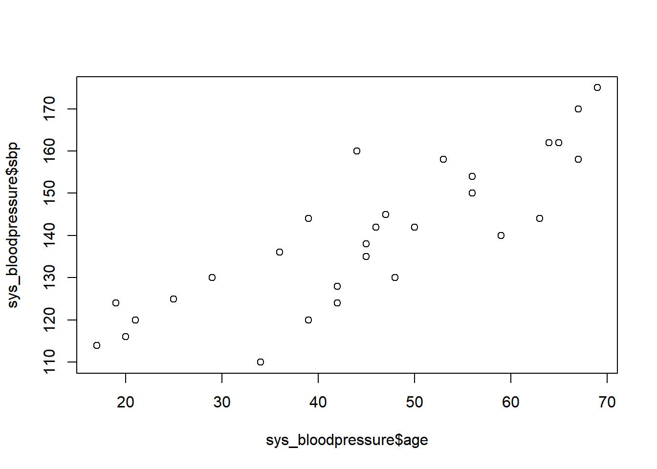
Then we see that the observation with the systolic blood pressure of 220 is no longer there. Now that we have checked that our data is correct, we can proceed to linear regression with the glm() function. Then we indeed see that the observation with the systolic blood pressure of 220 is no longer there.
Now that we have checked that all our data is correct, we can proceed to the linear regression with the glm() function.
The code to perform the glm() function is quite simple. All we have to do is specify a regression formula, a family argument, and optionally a data argument. If we type ?glm we can read the documentation and learn more about what arguments there are and what they are used for.
If we want to specify a formula, we need to use the “tilde” character ~ that we have seen one chapter earlier. We should start with the outcome variable (or dependent variable), followed by the tilde character, and then one or more independent variables.
Next, we have the family argument, and since we want to perform linear regression we should set this to “gaussian”. Optionally, we can specify a data argument. If we specify the data argument, then we don’t need to index the data all the time and we can just use the name of the columns from the data.
We type in the following code to perform the linear regression:
regression <- glm(sbp ~ age, family = "gaussian", data = sys_bloodpressure)In this case, we have performed the linear regression, and it is stored in the variable called regression. Now what we can do is use the summary() function on our regression variable, and then we can see the results of our linear regression.
summary(regression)##
## Call:
## glm(formula = sbp ~ age, family = "gaussian", data = sys_bloodpressure)
##
## Deviance Residuals:
## Min 1Q Median 3Q Max
## -19.354 -4.797 1.254 4.747 21.153
##
## Coefficients:
## Estimate Std. Error t value Pr(>|t|)
## (Intercept) 97.0771 5.5276 17.562 2.67e-16 ***
## age 0.9493 0.1161 8.174 8.88e-09 ***
## ---
## Signif. codes: 0 '***' 0.001 '**' 0.01 '*' 0.05 '.' 0.1 ' ' 1
##
## (Dispersion parameter for gaussian family taken to be 91.45728)
##
## Null deviance: 8579.4 on 28 degrees of freedom
## Residual deviance: 2469.3 on 27 degrees of freedom
## (1 observation deleted due to missingness)
## AIC: 217.19
##
## Number of Fisher Scoring iterations: 2We see several things here with the first one being “call”. Call is the formula we have specified to get these results. We also see deviance residuals, and these give information about the residuals. The coefficients are the most important thing here. We see an intercept and a coefficient for age here. Additionally, we also see the standard errors, t-values, and p-values for these coefficients. The significance is indicated by the number of asterisks as well.
The interpretation of these coefficients is that the systolic blood pressure increases by 0.94 for every 1-year increase in age. The intercept is hypothetical but applies to people who have an age of 0, and they would have a systolic blood pressure of 97.
In the output, we see in parentheses that 1 observation was removed because it was missing. If you use the glm() function and there are NA’s in your data, they will automatically be removed from the regression. This is because of the na.action argument of the glm() function which is by default set to na.omit. This means that the NA values will be removed.
The data argument
Earlier, we said that the data argument was optional and was not necessary. If we type in the following code:
Then we get the same result, but the difference is that we now have to specify the data for each variable. If you do specify the data argument then you don’t need to index the data all the time. You can imagine that if you want to perform a regression with ten independent variables it would be easier to specify the data argument.
Extension with multiple variables
In the example, we performed linear regression with only one independent variable. We refer to multiple linear regression if we want to use more than one independent variable. To perform multiple linear regression, we need to adjust the regression formula. For example, if we also had BMI in the dataset and we would like to use it as an independent variable as well, then we still specify the outcome variable, followed by the “tilde” sign, and then we type the independent variables separated by the + sign.
That will look like this:
regression2 <- glm(sbp ~ age + bmi, family = "gaussian", data = sys_bloodpressure)10.2 Logistic regression
Apart from linear regression, we can also perform logistic regression, and this is very similar to what we did for linear regression. Logistic regression is used when the outcome is a binary measurement (for example, dead/alive) as opposed to continuous measurements for linear regression.
This time, we will look at an example with myocardial infarction (mi). We will investigate whether there is a relationship between smoking and getting a heart attack (mi). First of all, we will start by loading the data (in this case, an SPSS file called mi).
library(foreign)
mi <- read.spss("mi.sav", to.data.frame = TRUE)
## re-encoding from UTF-8Of course, we can look at what kind of variables we have and what the first few observations look like:
head(mi)## pt_id mi smoking alcohol active sex profession
## 1 1 Patient Yes non-drinker Inactive male Epidemiologist
## 2 2 Patient Yes non-drinker Inactive male Statistician
## 3 4 Patient Yes non-drinker Active male Statistician
## 4 5 Patient No non-drinker Inactive male Epidemiologist
## 5 6 Patient No 1-2 glasses per day Active male Epidemiologist
## 6 7 Patient No non-drinker Inactive male Other
## bmi sys dias
## 1 24.70633 130 80
## 2 25.10582 160 100
## 3 26.39181 135 80
## 4 24.84901 120 90
## 5 24.25124 140 85
## 6 21.97494 120 80We see that there are 10 columns, but for this example, we will only use the second and third columns. Mi indicates if someone got a heart attack (patient) or not (control), and smoking shows whether the patients were smokers or non-smokers.
This dataset consists of 210 cases (patients) and 210 controls (case-control research). Therefore, there are 420 observations in total.
dim(mi)## [1] 420 10If we want to perform logistic regression, then we can use the glm() function again. Just like we did for linear regression, we should specify a regression formula, a family argument, and optionally a data argument. The only difference to perform linear regression and logistic regression is the family argument. In linear regression, we specified “gaussian” as the family argument, whereas we should specify “binomial” to perform logistic regression. So we type the following:
model <- glm(mi ~ smoking, family = "binomial", data = mi)Once we have done that, we can look at the results of the logistic regression by using the summary() function again. This time, we have stored the results in the variable called model. So, if we want to see the results, we should type summary(model):
summary(model)##
## Call:
## glm(formula = mi ~ smoking, family = "binomial", data = mi)
##
## Deviance Residuals:
## Min 1Q Median 3Q Max
## -1.45331 -1.10565 -0.09052 1.25090 1.25090
##
## Coefficients:
## Estimate Std. Error z value Pr(>|z|)
## (Intercept) -0.1711 0.1108 -1.544 0.12255
## smokingYes 0.7998 0.2454 3.260 0.00112 **
## ---
## Signif. codes: 0 '***' 0.001 '**' 0.01 '*' 0.05 '.' 0.1 ' ' 1
##
## (Dispersion parameter for binomial family taken to be 1)
##
## Null deviance: 582.24 on 419 degrees of freedom
## Residual deviance: 571.19 on 418 degrees of freedom
## AIC: 575.19
##
## Number of Fisher Scoring iterations: 4Here we see all the results of our logistic regression. The coefficients are now on a logit scale, and for those who have worked with logistic regression before, we know that we can change these coefficients to odds ratios by using the power of e. With Odds ratios, we can interpret these results.
This also allows us to look at how we can extract specific results from this regression. If we look at the Global environment after we have loaded the data and executed the regression, we can find the data and the model there.
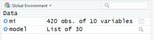
Figure 10.1: Global environemnt mi/model
The model has a list of 30 things in it. If we click on it (not on the arrow) but either on model or on the list of 30 a new screen called model will open. On this screen, you will find all the results in a list, and we can extract these results as well.
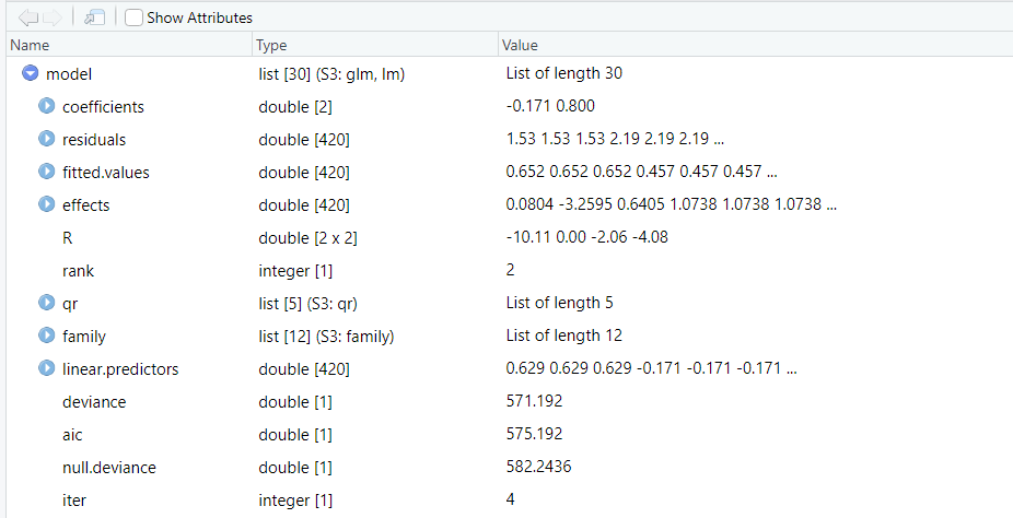
Figure 10.2: List model
In the list, we will find the coefficients, and in the column next to it, we see what type of values these are and what values are in it. In this way, we can extract these values as well. If we type model$ coefficients:
model$coefficients## (Intercept) smokingYes
## -0.1711483 0.7997569then we will see the coefficients for intercept and smoking. If we are only interested in smoking, then we can only index that coefficient. The coefficient for smoking is in the second position, so if we want to extract it, we can type model$coefficients[2].
model$coefficients[2]## smokingYes
## 0.7997569Now we only have the coefficient for smoking. If we want to use the power of e to turn this coefficient into an odds ratio, we can use the exp() function.
exp(model$coefficients[2])## smokingYes
## 2.225And this is the Odds ratio for smoking. If you want to interpret this odds ratio you should pay attention to the reference category. In this case, the reference category is non-smokers and the coefficient applies to smokers (also shown in smokingYes). This means that smokers have 2.25 higher odds of getting a heart attack compared to non-smokers. This result is significant because we could see that the coefficient for smoking had a p-value of < 0.05 (0.00112). For this example, we only extracted the coefficients from the list, but similarly, you can extract the other information as well.
10.3 Other types of regression
In this chapter, we have shown how we can perform both linear regression and logistic regression, but we can also perform other types of regression. The glm() function makes it easy to perform other regression types since the only difference is the “family” argument. Besides gaussian for linear regression and binomial for logistic regression, we can also specify “poisson” to the family argument to perform a poisson regression. The rest of the possible family arguments can be found in the documentation if you run ?family.
?family10.4 Predict function
If we have made a regression model with the glm() function, we can also make predictions. To illustrate this, we use the regression model called regression that we made earlier, and we will load new data to make predictions.
We start by loading our new data. In this case, it is a CSV file called new_age.
new_age <- read.csv("new_age.csv")If we type new_age we will see the new data.
new_age## age sbp
## 1 67 150
## 2 68 160
## 3 69 170
## 4 70 164
## 5 80 180
## 6 90 179We have six observations with age and the corresponding systolic blood pressure of persons. Now what we are going to do is make a prediction based on the age variable, and since we have real values of the systolic blood pressure, we can compare the predictions to the real values later on.
We can make predictions with the predict() function, and this function takes as arguments a model and new data. For now, we will save these predictions as predictions_sbp.
predictions_sbp <- predict(regression, newdata = new_age)If we then look at the predictions by executing predictions_sbp:
predictions_sbp## 1 2 3 4 5 6
## 160.6817 161.6310 162.5803 163.5297 173.0229 182.5161Then we will see the predicted systolic blood pressure for each person. These predictions were based on the age variable from the new data (67 to 70, 80, and 90). Recall that our regression model had an intercept of 97.0770843 and a coefficient for age of 0.9493225.
regression$coefficients## (Intercept) age
## 97.0770843 0.9493225That means that we could’ve also made these predictions ourselves. For example, if we want to predict the systolic blood pressure for a person with the age of 67, then it will look like this:
97.0770843 + (0.9493225 * 67)## [1] 160.6817And this corresponds with the first value of predictions_sbp.
Now that we have the predictions, we can see how good these predictions are when we compare them to the real systolic blood pressure values.
For linear regression, we can assess how good the predictions are based on several values, such as the mean squared error (MSE), mean absolute error (MAE), and root mean squared error (RMSE). These values can be obtained by using the Metrics package, which has functions to calculate all these values.
For now, I will only show how we can get the MSE and the RMSE since the code for the MAE is identical except for the fact that we have to use the mae() function instead of the mse() and rmse() functions.
We will start by loading the Metrics package (make sure you have installed it first before loading it with library()):
library(Metrics)If we want to know the mean squared error, we can use the mse() function. This function takes as arguments: actual for the real values and predicted for the predicted values. In our case, we will execute the following code to get the mean squared error:
mse(actual = new_age$sbp, predicted = predictions_sbp)## [1] 38.84576To obtain the RMSE function, we can do the same. Again, we specify actual and predicted as arguments, and then will get the RMSE.
rmse(actual = new_age$sbp, predicted = predictions_sbp)## [1] 6.232636This RMSE can be interpreted as follows: On average, the predictions are off by 6.23 units of systolic blood pressure. Also, the name indicates that the RMSE is the square root of the MSE but the advantage is that the interpretation from the RMSE is units of the outcome.
We can also make predictions with our logistic regression model. However, for this, we will need some extra steps. We will use our logistic regression model to predict based on the smoking variable, whether a person will have a heart attack or not.
Again, we need to load new data:
new_smoking <- read.csv("new_smoking.csv")new_smoking## smoking mi
## 1 Yes Patient
## 2 Yes Patient
## 3 Yes Patient
## 4 No Patient
## 5 No Control
## 6 No Control
## 7 Yes Patient
## 8 No Patient
## 9 Yes Patient
## 10 No Control
## 11 Yes Patient
## 12 Yes Patient
## 13 No Control
## 14 Yes PatientFor this example, we have 14 observations with a table whether someone is a smoker (yes) or a non-smoker (no), and whether someone had a heart attack (Patient) or not (Control).
Now we can do the same thing as we did for linear regression with the only difference that we need to give an extra argument called “type” to obtain the predicted chances.
For now, we will call these predictions predictions:
predictions <- predict(model, newdata = new_smoking, type = "response")
predictions
## 1 2 3 4 5 6 7 8
## 0.6521739 0.6521739 0.6521739 0.4573171 0.4573171 0.4573171 0.6521739 0.4573171
## 9 10 11 12 13 14
## 0.6521739 0.4573171 0.6521739 0.6521739 0.4573171 0.6521739If we look at the predictions, we see that these numbers are the predicted chance of getting a heart attack based on the smoking variable. This means that we are not quite there yet because we are interested in the classification if someone will get a heart attack or not.
To obtain these classifications, we can use an ifelse statement. We have not used an ifelse statement before, but it is relatively simple. If we look at the code below:
classifications <- ifelse(predictions > 0.5, "Patient", "Control")we see that if the predicted chances are higher than 0.5, then we assign “Patient” and if they are lower than 0.5, we assign “Control”. For this example, we used a cut-off value of 0.5, but we could’ve also used other values.
If we look at the classifications, we can see that we have predicted based on the smoking variable whether or not someone will get a heart attack or not.
classifications## 1 2 3 4 5 6 7 8
## "Patient" "Patient" "Patient" "Control" "Control" "Control" "Patient" "Control"
## 9 10 11 12 13 14
## "Patient" "Control" "Patient" "Patient" "Control" "Patient"Now we can compare these predictions to the actual outcome. For this, we can use the table() function, and we can create a confusion matrix with the caret library.
First, we load the caret library:
library(caret)Next, we create a cross-table with the predictions and actual values by specifying the predicted argument for the predictions and actual for the actual values with the table() function:
cross_table = table(predicted = classifications, actual = new_smoking$mi)Now, if we look at our cross-table:
cross_table## actual
## predicted Control Patient
## Control 4 2
## Patient 0 8We can see the predicted outcomes and actual outcomes. The more often the predictions match with the actual outcomes, the better the predictions. Normally, it is useful to have the “event” as the first column, but we can solve this with the confusionMatrix() function. This is important because otherwise, you get different values for sensitivity and specificity. The confusionMatrix() functions a cross-table and an argument called “positive” as arguments. With this “positive” argument, you can indicate the event. In this case, the event is Patient since they received a heart attack.
confusionMatrix(cross_table, positive = "Patient")## Confusion Matrix and Statistics
##
##          actual
## predicted Control Patient
##   Control       4       2
##   Patient       0       8
##
## Accuracy : 0.8571
## 95% CI : (0.5719, 0.9822)
## No Information Rate : 0.7143
## P-Value [Acc > NIR] : 0.1904
##
## Kappa : 0.6957
##
## Mcnemar's Test P-Value : 0.4795
##
## Sensitivity : 0.8000
## Specificity : 1.0000
## Pos Pred Value : 1.0000
## Neg Pred Value : 0.6667
## Prevalence : 0.7143
## Detection Rate : 0.5714
## Detection Prevalence : 0.5714
## Balanced Accuracy : 0.9000
##
## 'Positive' Class : Patient
## This confusion matrix gives a lot of information about the predictions with accuracy, sensitivity, specificity, positive and negative predicted values to name a few.