3 Day 3 (January 24)

3.1 Announcements

• Please read (and re-read) Chs. 2-3 in BBM2L
  • Library should have electronic copy soon
• Assignment 2 is posted and due Sunday Jan. 29
  • Start it before class on Thursday
• How I normally grade assignments
  • I will release a guide after I grade if needed
  • You will get an opportunity to improve your grade by explaining in detail why your work is different from mine the guide
  • Don’t hand in late, incomplete, or low effort work
  • May go over details in class
• Assignment 1
  • Overall great work!
  • Reproducible vs. too much output
  • Chi-squared distribution with 1 degree of freedom
  • Plots/figures
    • Clearly label what is being shown (e.g., frequency vs. density)
    • Write a very short figure legend
    • Have a friend see if they can determine what is being shown

3.2 Intro to Bayesian statistical modelling

• Example: my retirement

  • We developed a statistical model using tools approved by Reverend Bayes (i.e., the prior predictive distribution).
  • We selected a computational algorithm to preform Monte Carlo sampling from the prior predictive distribution.
  • We summarized samples from the prior predictive distribution in a way that helped us solve the problem at hand.

• Example: Estimating the population growth rate of the endangered whooping crane

  • Motivating data example

  url <- "https://www.dropbox.com/s/sr2411umm053vcq/Butler%20et%20al.%20Table%201.csv?dl=1"
  df1 <- read.csv(url)
  plot(df1$Winter, df1$N, typ = "b", xlab = "Year", ylab = "Population Size", 
  ylim = c(0, 300), lwd = 1.5, pch = "*")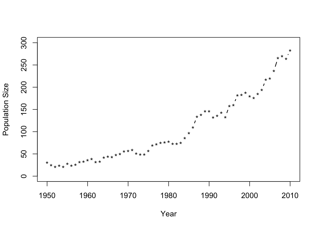

  

  • Statistical model \[y_t\sim~\text{Poisson}(\lambda(t))\] where \[\lambda(t)=\lambda_{0}e^{\gamma(t-t_0)}\]
    • Assume \(\lambda_0\) is known and equal to the the population size in 1950 (\(\lambda_0 = 31\))
    • We want to obtain the distribtuion of \(\gamma\) given the data \(\mathbf{y}\)
    • What else do we need to fully specify the model?

  K <- 10^6                   # Number of samples to try  
  samples <- matrix(,K,2)     # Save samples
  lambda0 <- df1$N[1]         # Lambda0
  y <- df1$N[-1]              # Data
  t <- df1$Winter[-1] - 1950  # Time
  
  for(i in 1:K){
  
    gamma <- runif(1,0,0.1)
    lambda <- lambda0*exp(gamma*t)
    y.sample <- rpois(length(t),lambda)
  
    samples[i,1] <- mean(abs(y-y.sample))
    samples[i,2] <- gamma
  }
  
  par(mfrow=c(1,2))
  hist(samples[,2],col="grey", main="Prior distribution",xlab=expression(gamma),ylab=expression("["*gamma*"]"),ylim=c(0,100),freq=FALSE,breaks=seq(0,0.1,by=0.005))
  hist(samples[which(samples[,1]<30),2],ylim=c(0,100),xlim=range(samples[,2]),col="grey", main="Posterior distribution",xlab=expression(gamma*"|"*bold(y)),ylab=expression("["*gamma*"|"*bold(y)*"]"),freq=FALSE,breaks=seq(0,0.1,by=0.005))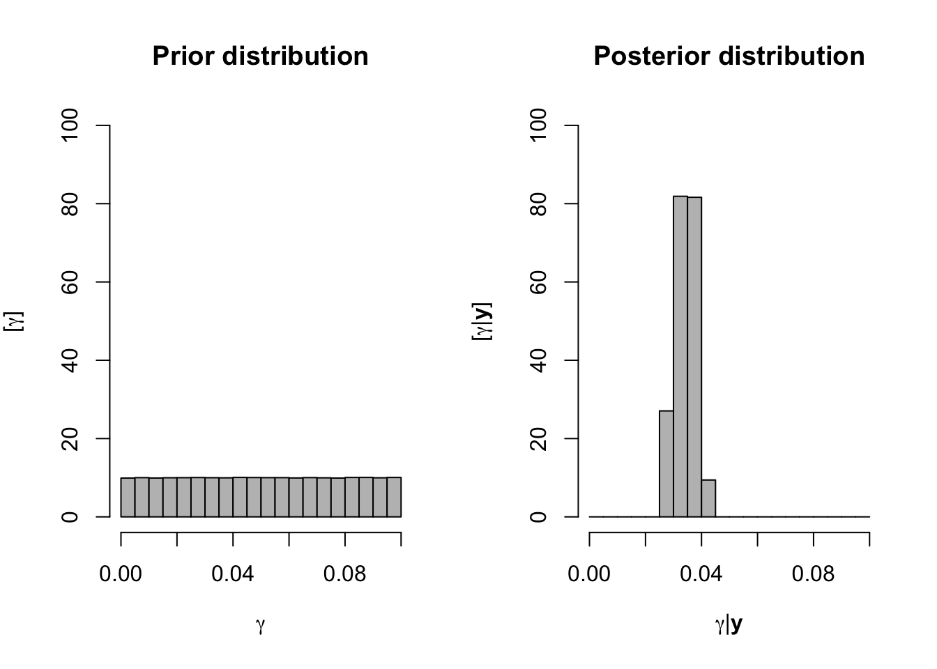 

  

• Example: Mississippi river restoration program

  • pdf