12 Day 12 (February 28)

12.1 Announcements

Status update on proposals and projects
Assignment 5 grades
Zoom office hours today
- Changed to 2-3 pm (Usually 1-2pm)
Questions about Assignment 6?
- More time?
Read Ch. 11 on Linear Regression
Read Ch. 12 on Posterior Prediction
- Funny and relevant

12.2 The Bayesian Linear Model

The model
- Distribution of the data: “\(\mathbf{y}\) given \(\boldsymbol{\beta}\) and \(\sigma_{\varepsilon}^{2}\)” \[[\mathbf{y}|\boldsymbol{\beta},\sigma_{\varepsilon}^{2}]\equiv\text{N}(\mathbf{X}\boldsymbol{\beta},\sigma_{\varepsilon}^{2}\mathbf{I})\] This is also sometimes called the data model.
- Distribution of the parameters: \(\boldsymbol{\beta}\) and \(\sigma_{\varepsilon}^{2}\) \[[\boldsymbol{\beta}]\equiv\text{N}(\mathbf{0},\sigma_{\beta}^{2}\mathbf{I})\] \[[\sigma_{\varepsilon}^{2}]\equiv\text{inverse gamma}(q,r)\]
Computations and statistical inference
- Using Bayes rule (Bayes 1763) we can obtain the joint posterior distribution \[[\boldsymbol{\beta},\sigma_{\varepsilon}^{2}|\mathbf{y}]=\frac{[\mathbf{y}|\boldsymbol{\beta},\sigma_{\varepsilon}^{2}][\boldsymbol{\beta}][\sigma_{\varepsilon}^{2}]}{\int\int [\mathbf{y}|\boldsymbol{\beta},\sigma_{\varepsilon}^{2}][\boldsymbol{\beta}][\sigma_{\varepsilon}^{2}]d\boldsymbol{\beta}d\sigma_{\varepsilon}^{2}}\]
  - Statistical inference about a parameters is obtained from the marginal posterior distributions \[[\boldsymbol{\beta}|\mathbf{y}]=\int[\boldsymbol{\beta},\sigma_{\varepsilon}^{2}|\mathbf{y}]d\sigma_{\varepsilon}^{2}\] \[[\sigma_{\varepsilon}^{2}|\mathbf{y}]=\int[\boldsymbol{\beta},\sigma_{\varepsilon}^{2}|\mathbf{y}]d\boldsymbol{\beta}\]
- In practice it is difficult to find closed-form solutions for the marginal posterior distributions, but easy to find closed-form solutions for the conditional posterior distribtuions.
  - Full-conditional distribtuions: \(\boldsymbol{\beta}\) and \(\sigma_{\varepsilon}^{2}\) \[[\boldsymbol{\beta}|\sigma_{\varepsilon}^{2},\mathbf{y}]\equiv\text{N}\bigg{(}\big{(}\mathbf{X}^{\prime}\mathbf{X}+\frac{1}{\sigma_{\beta}^{2}}\mathbf{I}\big{)}^{-1}\mathbf{X}^{\prime}\mathbf{y},\sigma_{\varepsilon}^{2}\big{(}\mathbf{X}^{\prime}\mathbf{X}+\frac{1}{\sigma_{\beta}^{2}}\mathbf{I}\big{)}^{-1}\bigg{)}\] \[[\sigma_{\varepsilon}^{2}|\mathbf{\boldsymbol{\beta}},\mathbf{y}]\equiv\text{inverse gamma}\left(q+\frac{n}{2},(r+\frac{1}{2}(\mathbf{y}-\mathbf{X}\boldsymbol{\beta})^{'}(\mathbf{y}-\mathbf{X}\boldsymbol{\beta}))^-1\right)\]
  - How do you find the full-conditional distributions for the Bayesian linear model?
    - \([\boldsymbol{\beta}|\sigma_{\varepsilon}^{2},\mathbf{y}]\)
    - \([\sigma_{\varepsilon}^{2}|\boldsymbol{\beta},\mathbf{y}]\)
  - Gibbs sampler for the Bayesian linear model
    - Write out on the whiteboard

Example: Mauna Loa Observatory carbon dioxide data

url <- "ftp://aftp.cmdl.noaa.gov/products/trends/co2/co2_annmean_mlo.txt" 
df <- read.table(url,header=FALSE) 
colnames(df) <- c("year","meanCO2","unc")
plot(x = df$year, y = df$meanCO2, xlab = "Year", ylab = expression("Mean annual "*CO[2]*" concentration"),col="black",pch=20)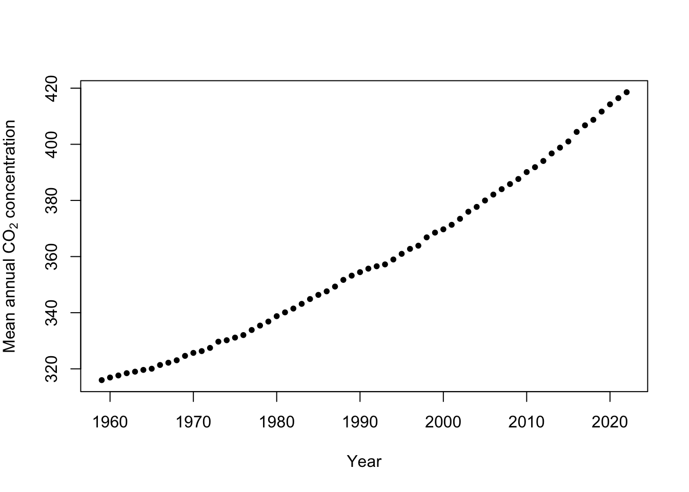

Gibb sampler

# Preliminary steps
library(mvnfast) # Required package to sample from multivariate normal distribution

y <- df$meanCO2 # Response variable
X <- model.matrix(~year, data=df) # Design matrix
n <- length(y) # Number of observations
p <- 2 # Dimensions of beta

K <- 5000  #Number of MCMC samples to draw

samples <- as.data.frame(matrix(,K,3)) # Samples of the parameters we will save
colnames(samples) <- c(colnames(X),"sigma2")

sigma2.e <- 1  # Starting values for sigma2

sigma2.beta <- 10^6 #Prior variance for beta
q <- 2.01 #Inverse gamma prior with E() = 1/(r*(q-1)) and Var()= 1/(r^2*(q-1)^2*(q-2))
r <- 1


# MCMC algorithm
for(k in 1:K){
  # Sample beta from full-conditional distribution
  H <- solve(t(X)%*%X + diag(1/sigma2.beta,p))
  h <- t(X)%*%y
  beta <-  t(rmvn(1,H%*%h,sigma2.e*H))

  # Sample sigma from full-conditional distribution
  q.temp <- q+n/2
  r.temp <- (1/r+t(y-X%*%beta)%*%(y-X%*%beta)/2)^-1
  sigma2.e <- 1/rgamma(1,q.temp,,r.temp)

  # Save samples of beta and sigma
  samples[k,] <- c(beta,sigma2.e)
}


burn.in <- 1000

# Look a histograms of posterior distributions
par(mfrow=c(3,1),mar=c(5,6,1,1))
hist(samples[-c(1:burn.in),1],xlab=expression(beta[0]*"|"*bold(y)),ylab=expression("["*beta[0]*"|"*bold(y)*"]"),freq=FALSE,col="grey",main="",breaks=30)
hist(samples[-c(1:burn.in),2],xlab=expression(beta[1]*"|"*bold(y)),ylab=expression("["*beta[1]*"|"*bold(y)*"]"),freq=FALSE,col="grey",main="",breaks=30)
hist(samples[-c(1:burn.in),3],xlab=expression(sigma^2*"|"*bold(y)),ylab=expression("["*sigma^2*"|"*bold(y)*"]"),freq=FALSE,col="grey",main="",breaks=30)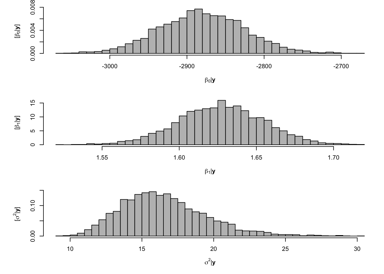

# Expected value of the posterior distribution
colMeans(samples[-c(1:burn.in),])

##  (Intercept)         year       sigma2 
## -2880.261714     1.627009    16.536422

# 95 % equal-tailed credible interval
apply(samples[-c(1:burn.in),],2,,FUN=quantile,prob=c(0.025,0.975))

##       (Intercept)     year   sigma2
## 2.5%    -2987.425 1.572301 11.71094
## 97.5%   -2771.481 1.680803 23.31802

# Compare to results obtained from lm function
m1 <- lm(y~X-1)
coef(m1)

## X(Intercept)        Xyear 
## -2881.924866     1.627842

confint(m1)

##                     2.5 %       97.5 %
## X(Intercept) -2992.978151 -2770.871581
## Xyear            1.572053     1.683632

summary(m1)$sigma^2

## [1] 17.01142

Using the R package MCMCpack

library(MCMCpack)
samples <- MCMCregress(y ~ X - 1,
                         burnin = 0,mcmc = 5000 ,
                         b0 = 0,B0 = 1/sigma2.beta,
                         c0 = q, d0 = 1/r)

burn.in <- 1000
samples <- samples[burn.in:5000,] # Extract samples from the posterior for beta and sigma2 from MCMCregress output

# Look a histograms of posterior distributions
par(mfrow=c(3,1),mar=c(5,6,1,1))
hist(samples[,1],xlab=expression(beta[0]*"|"*bold(y)),ylab=expression("["*beta[0]*"|"*bold(y)*"]"),freq=FALSE,col="grey",main="",breaks=30)
hist(samples[,2],xlab=expression(beta[1]*"|"*bold(y)),ylab=expression("["*beta[1]*"|"*bold(y)*"]"),freq=FALSE,col="grey",main="",breaks=30)
hist(samples[,3],xlab=expression(sigma^2*"|"*bold(y)),ylab=expression("["*sigma^2*"|"*bold(y)*"]"),freq=FALSE,col="grey",main="",breaks=30)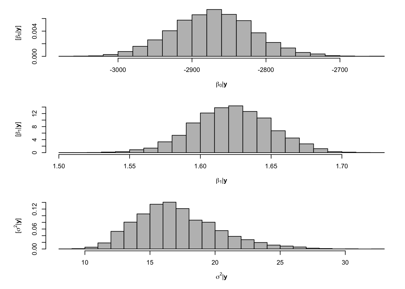

# Expected value of the posterior distribution
colMeans(samples)

## X(Intercept)        Xyear       sigma2 
## -2871.266552     1.622486    17.104495

# 95 % equal-tailed credible interval
apply(samples,2,,FUN=quantile,prob=c(0.025,0.975))

##       X(Intercept)    Xyear   sigma2
## 2.5%     -2978.058 1.568383 12.00651
## 97.5%    -2763.594 1.676256 24.38504

12.3 Bayesian Kriging

Modify the linear model
- Account for spatial autocorrelation
- Enable prediction at locations