2 Day 2 (January 19)

2.1 Announcements

Please read (and re-read) Chs. 1-2 in BBM2L before class next week
I will post assignment 2 by Monday
Remember that we are starting slow. Use the time wisely
More generative AI jokes
Donuts and meeting your peers
- Opportunity for 5 magical extra credit points

2.2 Intro to Bayesian statistical modelling

What is data?
- Something in the real world that you can, in some way, observe and measure with or without error
What is a statistic?
- A function of the data
What is a model?
- Mathematical models
- Statistical models
What is goal of Bayesian statistics?
- Obtain the distribution of potentially unrecordable random variables given recorded random variables

Example: my retirement

Personal information
- Obviously this isn’t my actual information, but it isn’t too far off!
- Since I am a millennial I don’t think social security will be around when I retire (i.e., assume social security contributes $0 to my retirement)
- As of 1/1/23 I have $100,000 in 401k retirement in accounts
- All of money is invested into an S&P 500 index fund (VOO to be exact)
- I am 35 as of 1/1/23
- I want to know how much pre-tax money I will have at a given retirement age (e.g., 65, 70, etc)
Example using a mathematical model
- Whiteboard demonstration
- What are the model assumptions?
- In program R

# The value of my 401k retirement account as of 1/1/23
y_2023 <- 100000 


# How much money will I add to my 401k each year
q <- 20000


# Rate of return for S&P 500 index fund
r <- 0.12


# How much $ will I have in 2024
y_2024 <- y_2023*(1+r)+q
y_2024

## [1] 132000

# How much $ will I have in 2025 
y_2025 <- y_2024*(1+r)+q
y_2025

## [1] 167840

# How much $ will I have in 2026 
y_2026 <- y_2025*(1+r)+q
y_2026

## [1] 207980.8

# Using a for loop to calculate how much $ will I have 
year <- seq(2023,2023+30,by=1)
y <- matrix(,length(year),1)
rownames(y) <- year
y[1,1] <- 100000

for(t in 1:30){
  y[t+1,1] <- y[t,1]*(1+r)+q
}

plot(year,y/10^6,typ="b",pch=20,col="deepskyblue",xlab="Year",ylab="Pretax retirement amount ($ millions)")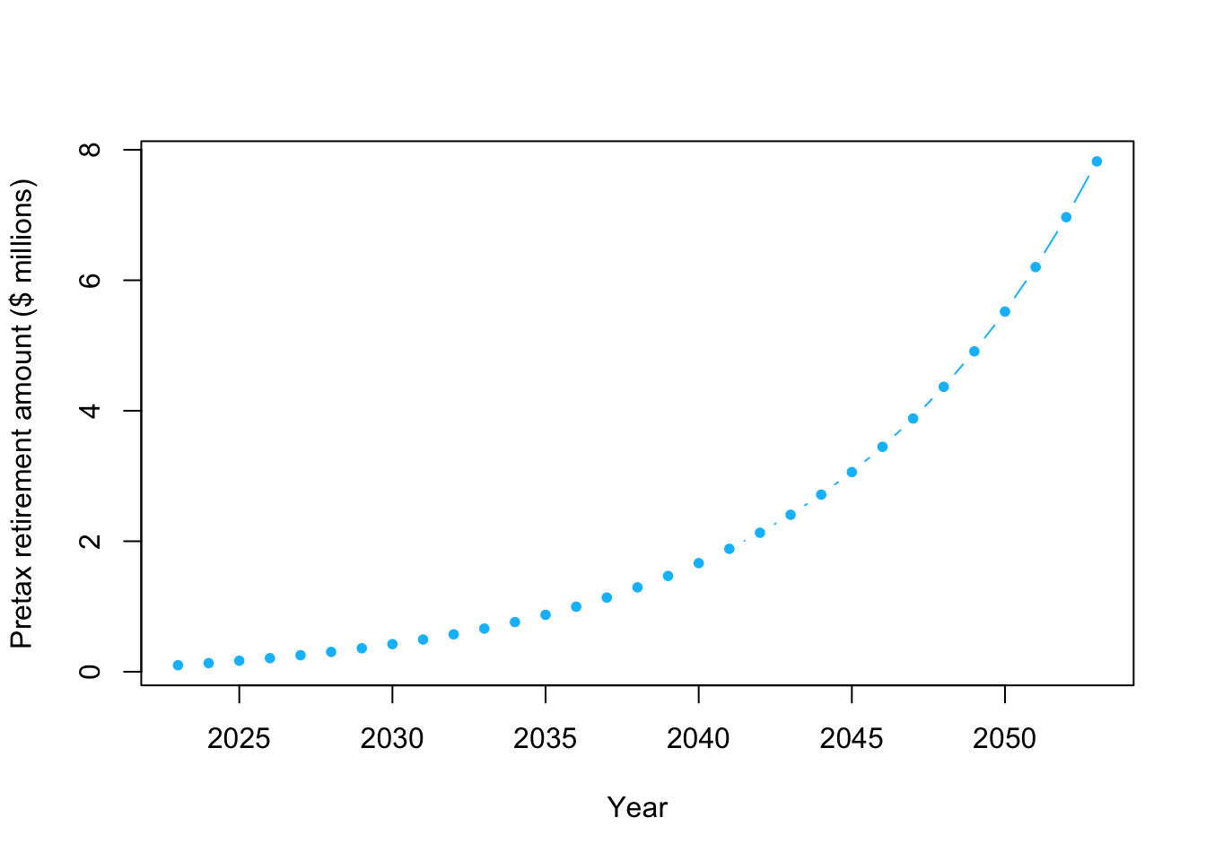

# How much $ will I have when I am 65? 
# Note that units are millions of $
retirement.year <- 2023+30
y[which(year==retirement.year)]/10^6

## [1] 7.822646

Example using a Bayesian statistical model
- Whiteboard demonstration
- S&P 500 return since inception in 1957

# Download S&P 500 returns    
url <- "https://www.dropbox.com/s/81ccahyuaas1zpd/s%26p500.csv?dl=1"
df.sp500 <- read.csv(url)

head(df.sp500)

##   year  return
## 1 2022 -0.1811
## 2 2021  0.2871
## 3 2020  0.1840
## 4 2019  0.3149
## 5 2018 -0.0438
## 6 2017  0.2183

mean(df.sp500$return)

## [1] 0.1152742

hist(df.sp500$return,main="",col="grey",xlab=" Return rate of S&P 500")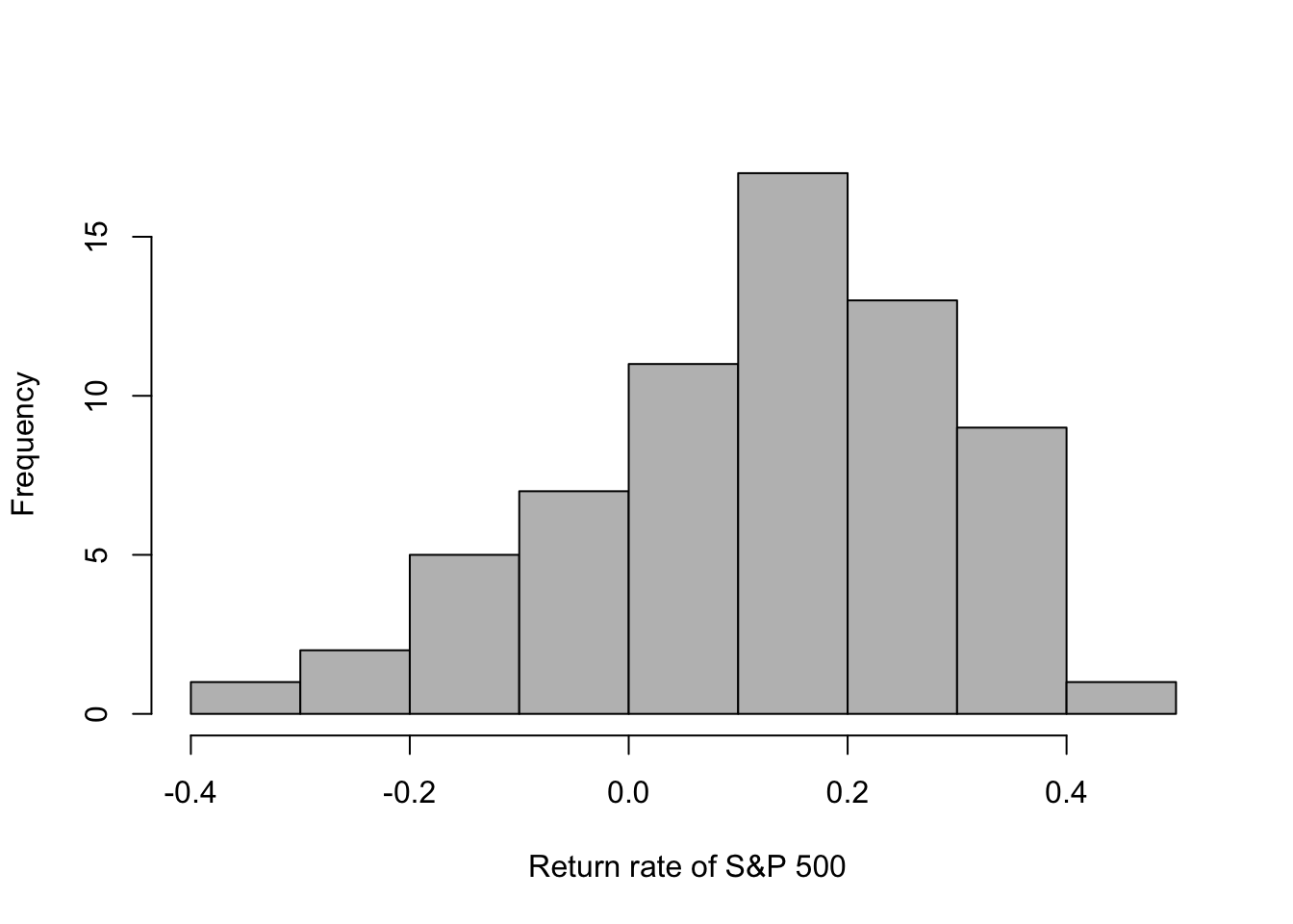

- Example using the prior predictive distribution

# Download S&P 500 returns
url <- "https://www.dropbox.com/s/81ccahyuaas1zpd/s%26p500.csv?dl=1"
df.sp500 <- read.csv(url)

# The value of my 401k retirement account as of 1/1/23
y_2023 <- 100000 

# How much money will I add to my 401k each year
q <- 20000


# Using a for loop to calculate how much $ will I have 
year <- seq(2023,2023+30,by=1)
Y <- matrix(,length(year),1000)
rownames(Y) <- year
Y[1,] <- y_2023

set.seed(3410)
for(m in 1:1000){
for(t in 1:30){
  r <- sample(df.sp500$return,1)
  Y[t+1,m] <- Y[t,m]*(1+r)+q
              }
                }


# Prior predictive distribution for a given year
retirement.year <- 2023+30
hist(Y[which(year==retirement.year),]/10^6,col="grey",freq=FALSE,xlab="Pretax retirement amount ($ millions)",main="")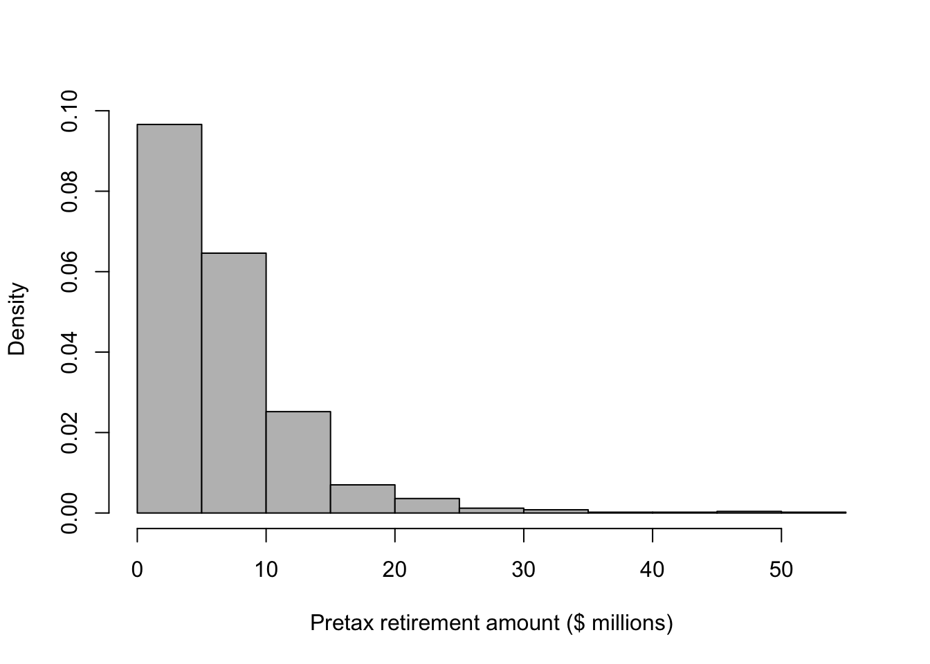

# Summary of prior predictive distribution
mean(Y[which(year==retirement.year),]/10^6)

## [1] 6.767347

max(Y[which(year==retirement.year),]/10^6)

## [1] 50.62067

min(Y[which(year==retirement.year),]/10^6)

## [1] 0.4278632

quantile(Y[which(year==retirement.year),]/10^6,probs=c(0.025,0.975))

##     2.5%    97.5% 
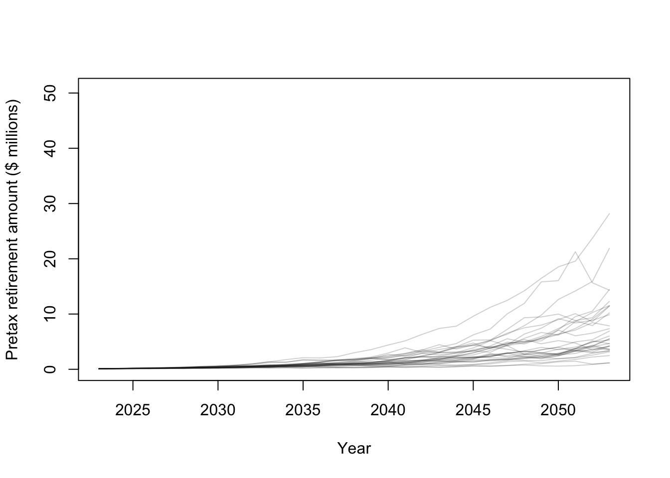
##  1.24744 21.41771

# Plot some financial trajectories (i.e., random draws from the prior predictive distribution)
plot(year,Y[,1]/10^6,typ="l",lwd=1,ylim=c(0,max(Y/10^6)),col=rgb(0.1,0.1,0.1,.2),xlab="Year",ylab="Pretax retirement amount ($ millions)") 
for(i in 1:30){
points(year,Y[,i]/10^6,typ="l",lwd=1,col=rgb(0.1,0.1,0.1,.2))
}

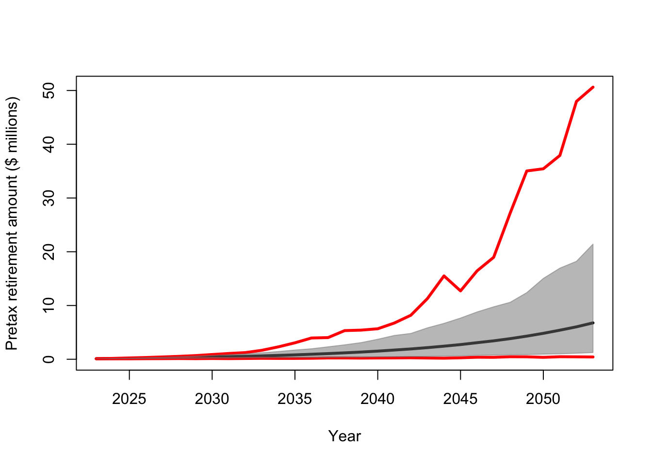
# Plot of prior predictive distribution for all years
E.Y <- apply(Y/10^6,1,mean)
u.CI <- apply(Y/10^6,1,quantile,prob=0.975)
l.CI <- apply(Y/10^6,1,quantile,prob=0.025)
max.Y <- apply(Y/10^6,1,max)
min.Y <- apply(Y/10^6,1,min)

plot(year,E.Y,typ="l",lwd=3,ylim=c(0,max(max.Y)),xlab="Year",ylab="Pretax retirement amount ($ millions)") 
points(year,max.Y,typ="l",lwd=3,col="red")
points(year,min.Y,typ="l",lwd=3,col="red")
polygon(c(year,rev(year)),c(u.CI,rev(l.CI)),
        col=rgb(0.5,0.5,0.5,0.5),border=rgb(0.5,0.5,0.5,0.5))