14 Day 14 (March 9)

14.1 Announcements

• Class projects

  • Proposal (submitted Feb. 17; All proposals have been retured)
  • Presentations will occur between May 2 and May 9
  • Peer review is due May 5
  • Report and reproducible analysis is due May 10

• Assignment 7 is posted and due Wednesday (March 22)

  • Short in-class demonstration

• Read Ch. 17 on spatial models

• Question about the Bayesian view of missing data

14.2 Bayesian Prediction

• Review how to do prediction using linear model

  • Difference between prediction intervals and confidence intervals?
  • Do we need an example using R?

• Derived derived quantities

  • Functions of one or more posterior distribution

• Predictive/forecast distributions vs. point estimate

  • Popular measures of predictive accuracy

• Posterior prediction vs. prior prediction

  • Remember the retirement example? (see here)

• What do we mean and what do we want to show when we make predictions?
  

• Posterior prediction

  • Use data/process model to determine the full-conditional distribution of the unobserved data given the parameters and observed data
  • Use composition sampling to perform integration in Eq. 12.2 to BBM2L

  # Preliminary steps
  library(mvnfast) # Required package to sample from multivariate normal distribution
  
  url <- "ftp://aftp.cmdl.noaa.gov/products/trends/co2/co2_annmean_mlo.txt" 
  df <- read.table(url,header=FALSE) 
  colnames(df) <- c("year","meanCO2","unc")
  
  y <- df$meanCO2 # Response variable
  X <- model.matrix(~year, data=df) # Design matrix
  n <- length(y) # Number of observations
  p <- 2 # Dimensions of beta
  
  K <- 5000  #Number of MCMC samples to draw
  
  samples <- as.data.frame(matrix(,K,3)) # Samples of the parameters we will save
  colnames(samples) <- c(colnames(X),"sigma2")
  
  sigma2.e <- 1  # Starting values for sigma2
  
  sigma2.beta <- 10^6 #Prior variance for beta
  q <- 2.01 #Inverse gamma prior with E() = 1/(r*(q-1)) and Var()= 1/(r^2*(q-1)^2*(q-2))
  r <- 1
  
  
  # MCMC algorithm
  for(k in 1:K){
    # Sample beta from full-conditional distribution
    H <- solve(t(X)%*%X + diag(1/sigma2.beta,p))
    h <- t(X)%*%y
    beta <-  t(rmvn(1,H%*%h,sigma2.e*H))
  
    # Sample sigma from full-conditional distribution
    q.temp <- q+n/2
    r.temp <- (1/r+t(y-X%*%beta)%*%(y-X%*%beta)/2)^-1
    sigma2.e <- 1/rgamma(1,q.temp,,r.temp)
  
    # Save samples of beta and sigma
    samples[k,] <- c(beta,sigma2.e)
  }
  
  
  burn.in <- 1000
  
  # Use composition sampling to take samples from 
  # the posterior predictive distribution
  year <- 2050
  K <- dim(samples)[1]
  beta0.y <- samples[,1]
  beta1.y <- samples[,2]
  sigma2.y <-samples[,3]
  ppd.samples <- rnorm(K,beta0.y + beta1.y*year, sqrt(sigma2.y))
  
  # Histogram of samples from the posterior predictive distribution
  hist(ppd.samples[-c(1:burn.in)],,xlab=expression(tilde(y)*"|"*bold(y)),ylab=expression("["*tilde(y)*"|"*bold(y)*"]"),freq=FALSE,col="grey",main="",breaks=30)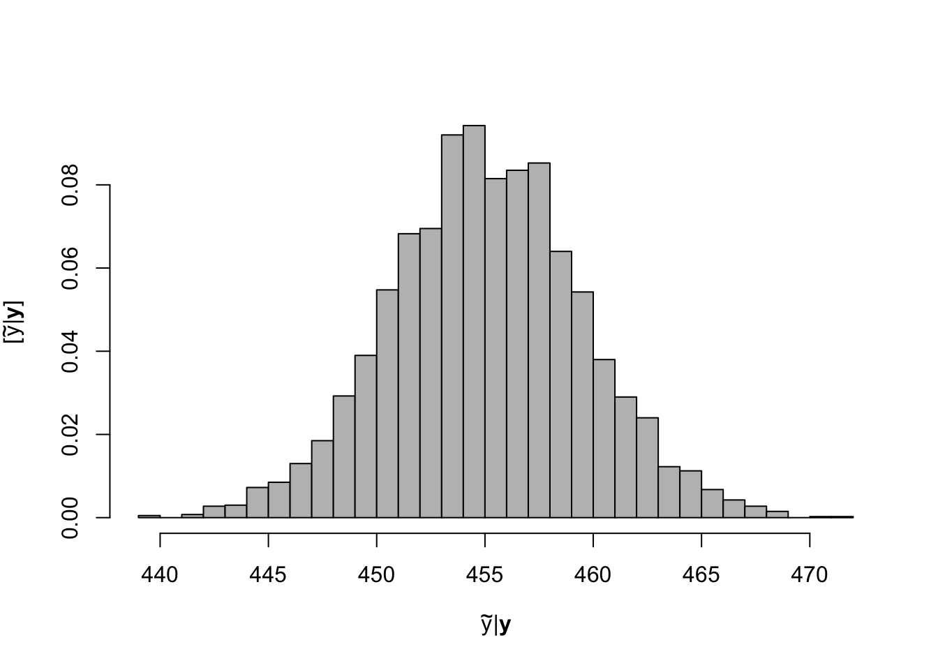

  

  # Expected value of the posterior predictive distribution
  mean(ppd.samples[-c(1:burn.in)])

  ## [1] 455.0655

  # 95 % equal-tailed credible interval
  quantile(ppd.samples[-c(1:burn.in)],prob=c(0.025,0.975))

  ##     2.5%    97.5% 
  ## 446.2166 464.1382

  # Compare to results obtained from lm function
  m1 <- lm(meanCO2~year,data=df)
  predict(m1,newdata=data.frame(year=2050),interval="prediction",level=0.95)

  ##        fit      lwr      upr
  ## 1 455.1518 446.2043 464.0992