16 Day 16 (March 23)
16.1 Announcements
- Assignment 7 is posted and due Sunday (March 26)
- Derived quantities
- Read Ch. 17 on spatial models
16.2 Gaussian process
- A Gaussian process is a probability distribution over functions
- If the function is observed at a finite number of points or “locations,” then the vector of values follows a multivariate normal distribution.
16.2.1 Multivariate normal distribution
Multivariate normal distribution
- \(\boldsymbol{\eta}\sim\text{N}(\mathbf{0},\sigma^{2}\mathbf{R})\)
- Definitions
- Correlation matrix – A positive semi-definite matrix whose elements are the correlation between observations
- Correlation function – A function that describes the correlation between observations
- Example correlation matrices
- Compound symmetry \[\mathbf{R}=\left[\begin{array}{cccccc} 1 & 1 & 0 & 0 & 0 & 0\\ 1 & 1 & 0 & 0 & 0 & 0\\ 0 & 0 & 1 & 1 & 0 & 0\\ 0 & 0 & 1 & 1 & 0 & 0\\ 0 & 0 & 0 & 0 & 1 & 1\\ 0 & 0 & 0 & 0 & 1 & 1 \end{array}\right]\]
- AR(1) \[\mathbf{R(\phi})=\left[\begin{array}{ccccc} 1 & \phi^{1} & \phi^{2} & \cdots & \phi^{n-1}\\ \phi^{1} & 1 & \phi^{1} & \cdots & \phi^{n-2}\\ \phi^{2} & \phi^{1} & 1 & \vdots & \phi^{n-3}\\ \vdots & \vdots & \vdots & \ddots & \ddots\\ \phi^{n-1} & \phi^{n-2} & \phi^{n-3} & \ddots & 1 \end{array}\right]\:\]
Example simulating from \(\boldsymbol{\eta}\sim\text{N}(\mathbf{0},\sigma^{2}\mathbf{R})\) in R
n <- 200
x <- 1:n
I <- diag(1, n)
sigma2 <- 1

library(MASS)
set.seed(2034)
eta <- mvrnorm(1, rep(0, n), sigma2 * I)
cor(eta[1:(n - 1)], eta[2:n])
## [1] -0.06408623acf(eta)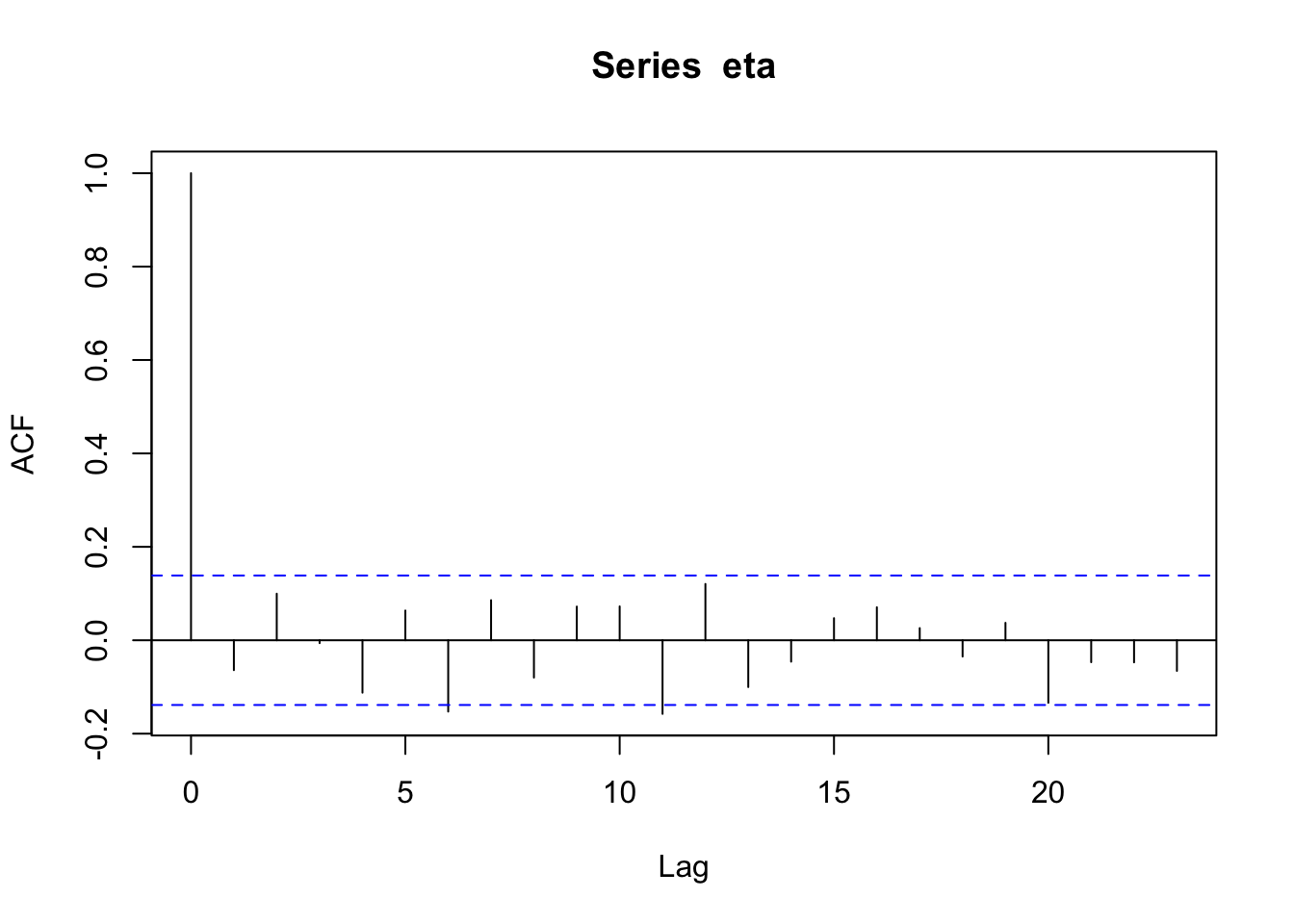
par(mfrow = c(2, 1))
par(mar = c(0, 2, 0, 0), oma = c(5.1, 3.1, 2.1, 2.1))
plot(x, eta, typ = "l", xlab = "", xaxt = "n")
abline(a = 0, b = 0)

n <- 200
x <- 1:n # Must be equally spaced
phi <- 0.7
R <- phi^abs(outer(x, x, "-"))
sigma2 <- 1
set.seed(1330)
eta <- mvrnorm(1, rep(0, n), sigma2 * R)
cor(eta[1:(n - 1)], eta[2:n])
## [1] 0.7016662plot(x, eta, typ = "l") abline(a = 0, b = 0)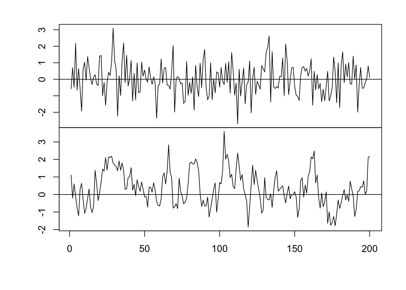
acf(eta)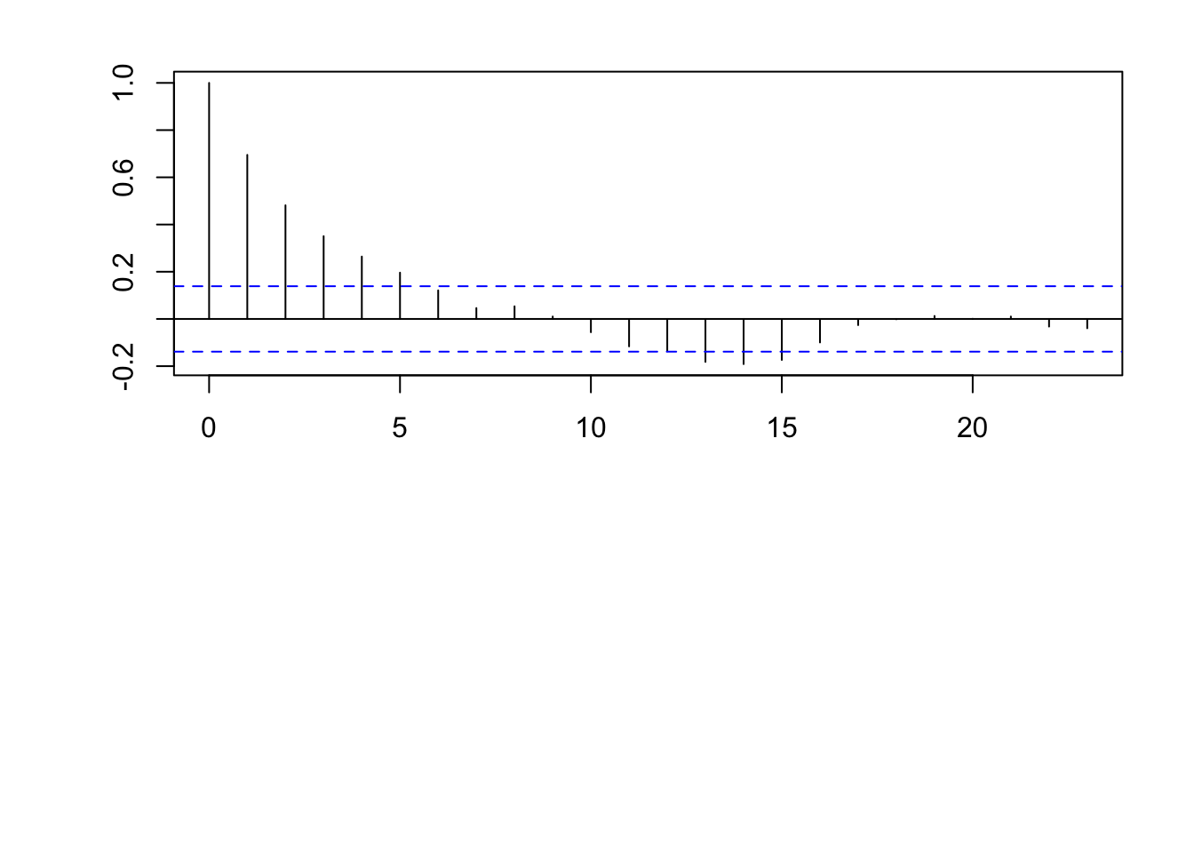
- Example correlation functions
- Gaussian correlation function \[r_{ij}(\phi)=e^{-\frac{d_{ij}^{2}}{\phi}}\] where \(d_{ij}\) is the “distance” between locations i and j (note that \(d_{ij}=0\) for \(i=j\)) and \(r_{ij}(\phi)\) is the element in the \(i^{\textrm{th}}\) row and \(j^{\textrm{th}}\) column of \(\mathbf{R}(\phi)\).
library(fields)
n <- 200
x <- 1:n
phi <- 40
d <- rdist(x)
R <- exp(-d^2/phi)
sigma2 <- 1

set.seed(4673)
eta <- mvrnorm(1, rep(0, n), sigma2 * R)
plot(x, eta, typ = "l")
abline(a = 0, b = 0)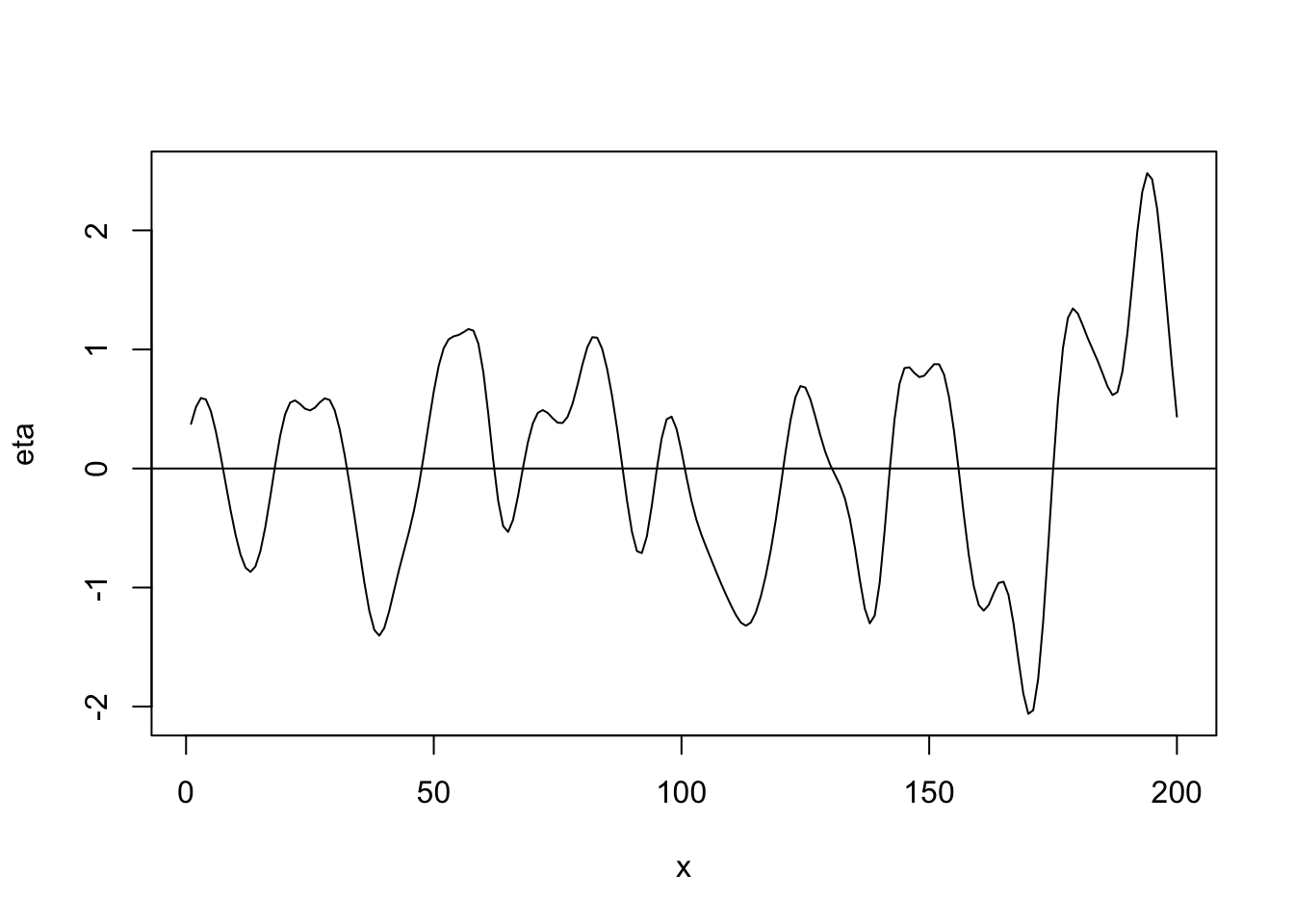
cor(eta[1:(n-1)], eta[2:n])## [1] 0.9713954- Linear correlation function \[r_{ij}(\phi)=\begin{cases} 1-\frac{d_{ij}}{\phi} &\text{if}\ d_{ij}<0\\ 0 &\text{if}\ d_{ij}>0 \end{cases}\]
library(fields)
n <- 200
x <- 1:n
phi <- 40
d <- rdist(x)
R <- ifelse(d<phi,1-d/phi,0)
sigma2 <- 1

set.seed(4803)
eta <- mvrnorm(1, rep(0, n), sigma2 * R)
plot(x, eta, typ = "l")
abline(a = 0, b = 0)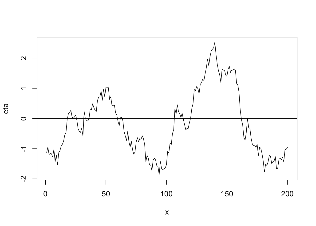
cor(eta[1:(n-1)], eta[2:n])## [1] 0.9775175- Example correlation functions
16.3 Bayesian Kriging
Read Chapter 17
Example data set
url <- "https://www.dropbox.com/s/k2ajjvyxwvsbqgf/ISIT.txt?dl=1"
df <- read.table(url, header = TRUE)
df <- df[df$Station == 16,c(1,2,5,6)]

head(df)
## Depth Sources Latitude Longitude ## 595 598 53.37 49.0322 -16.1493 ## 596 631 51.32 49.0322 -16.1493 ## 597 700 42.42 49.0322 -16.1493 ## 598 666 38.32 49.0322 -16.1493 ## 599 1317 37.29 49.0322 -16.1493 ## 600 1352 36.27 49.0322 -16.1493plot(df$Depth, df$Sources, las = 1, ylim = c(0, 65), col = rgb(0, 0, 0, 0.25), pch = 19, xlab = "Depth (m)", ylab = "Sources")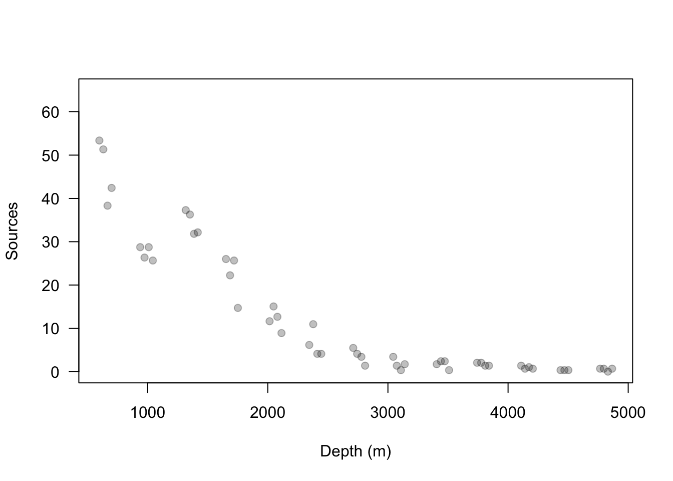
Modify the linear model
- Account for spatial autocorrelation
- Enable prediction at locations
- Write out on whiteboard
- In R
library(fields)
library(truncnorm)
library(mvtnorm)
library(coda)
library(MASS)

y <- df$Sources
X <- model.matrix(~I(Depth/Depth)-1,data=df)
Z <- diag(1,length(y))
n <- length(y)

# Distance matrix used to calculate correlation matrix
D <- rdist(df$Depth)

m.draws <- 10000  #Number of MCMC samples to draw
samples <- as.data.frame(matrix(,m.draws+1,dim(X)[2]+3))
colnames(samples) <- c(colnames(X),"sigma2.e","sigma2.alpha","phi")
samples[1,] <- c(40,10,150,250)  #Starting values for beta0, sigma2.e, sigma2.alpha, and phi
samples.alpha <- as.data.frame(matrix(,m.draws+1,length(y)))

# Hyperparameters for priors
sigma2.beta <- 100
a <- 2.01
b <- 1
c <- 2.01
d <- 1
e <- 0
f <- 10^6

accept <- matrix(, m.draws + 1, 1) # Monitor acceptance rate
colnames(accept) <- c("phi")
phi.tune <- 10

set.seed(3909)
ptm <- proc.time()
for(k in 1:m.draws){
  beta <- t(samples[k,1:dim(X)[2]])
  sigma2.e <- samples[k,dim(X)[2]+1]
  sigma2.alpha <- samples[k,dim(X)[2]+2]
  phi <- samples[k,dim(X)[2]+3]
  C <- exp(-(D/phi)^2)
  CI <- solve(C)

  # Sample alpha
  H <- solve((1/sigma2.e)*t(Z)%*%Z + (1/sigma2.alpha)*CI)
  h <- (1/sigma2.e)*t(Z)%*%(y-X%*%beta)
  alpha <-  mvrnorm(1,H%*%h,H)

  # Sample beta
  H <- solve((1/sigma2.e)*t(X)%*%X + (1/sigma2.beta)*diag(1,dim(X)[2]))
  h <- (1/sigma2.e)*t(X)%*%(y-Z%*%alpha)
  beta <-  mvrnorm(1,H%*%h,H)

  # Sample sigma2.alpha
  sigma2.alpha <- 1/rgamma(1,a+n/2,b+t(alpha)%*%CI%*%(alpha)/2)

  # Sample sigma2.e
  sigma2.e <- 1/rgamma(1,c+n/2,d+t(y-X%*%beta-Z%*%alpha)%*%(y-X%*%beta-Z%*%alpha)/2)

  #Sample phi
  phi.star <- rnorm(1,phi,phi.tune)
  if(phi.star > e & phi.star < f){
C.star <-  exp(-(D/phi.star)^2)
mh1 <- dmvnorm(alpha,rep(0,n),sigma2.alpha*C.star,log=TRUE) + dunif(phi.star,e,f,log=TRUE)
mh2 <- dmvnorm(alpha,rep(0,n),sigma2.alpha*C,log=TRUE) + dunif(phi,e,f,log=TRUE)
R <- min(1,exp(mh1 - mh2))
if (R > runif(1)){phi <- phi.star}}

  # Save
  samples[k+1,] <- c(beta,sigma2.e,sigma2.alpha,phi)
  samples.alpha[k+1,] <- alpha
  accept[k+1,] <- ifelse(phi==phi.star,1,0)
  if(k%%1000==0) print(k)
}
proc.time() - ptm

mean(accept[-1,])

par(mfrow=c(1,1),mar=c(5,5,2,2))
plot(samples[,1],typ="l",xlab="k",ylab=expression(beta[0]))
plot(samples[,2],typ="l",xlab="k",ylab=expression(sigma[epsilon]^2))
plot(samples[,3],typ="l",xlab="k",ylab=expression(sigma[alpha]^2))
plot(samples[,4],typ="l",xlab="k",ylab=expression(phi))

#Note: there is a trace plots for each of the 51 alphas
plot(samples.alpha[,1],typ="l",xlab="k",ylab=expression(alpha))

burn.in <- 1000

#Effective sample size
effectiveSize(samples[-c(1:burn.in),])
effectiveSize(samples.alpha[-c(1:burn.in),])

# E() of beta, sigma2.e, sigma2.alpha, phi
colMeans(samples[-c(1:burn.in),])

# 95% Equal-tailed CIs
apply(samples[-c(1:burn.in),],2,FUN=quantile,prob=c(0.025,0.975))


# obtain E(y) of at new depths
new.depth <- seq(min(df$Depth),max(df$Depth),by=10)
X.new <- model.matrix(~I(new.depth/new.depth)-1)
Z.new <- diag(1,length(new.depth))
D.cross <- rdist(new.depth,df$Depth)

samples.pred <- matrix(,length(burn.in:m.draws),length(new.depth))

for(k in burn.in:m.draws){
  alpha <- t(samples.alpha[k,])
  beta <- t(samples[k,1:dim(X)[2]])
  sigma2.e <- samples[k,dim(X)[2]+1]
  sigma2.alpha <- samples[k,dim(X)[2]+2]
  phi <- samples[k,dim(X)[2]+3]

  C <- exp(-(D/phi)^2)
  C.cross <- exp(-(D.cross/phi)^2)

  alpha.new <- C.cross%*%solve(C)%*%alpha
  samples.pred[k-burn.in+1,] <- X.new%*%beta + Z.new%*%alpha.new
}


plot(df$Depth,df$Sources,las=1,ylim=c(0,60),col=rgb(0,0,0,0.25),pch=19,
 xlab="Depth (m)",ylab="Sources")
points(new.depth,colMeans(samples.pred),typ="l")


EV.beta <- mean(samples[-c(1:burn.in),1])
EV.alpha <- colMeans(samples.alpha[-c(1:burn.in),])
EV.e <- y - X%*%EV.beta - Z%*%EV.alpha

par(mfrow=c(2,1))
plot(df$Depth, EV.e, las = 1, col = rgb(0, 0, 0, 0.25),pch = 19, xlab = "Depth (m)", ylab = expression("E("*epsilon*")"))
hist(EV.e,col="grey",main="",breaks=10,xlab= expression("E("*epsilon*")"))