Session 3 Tidy Up First

Data is the foundation of our visualisation/analysis workflow.

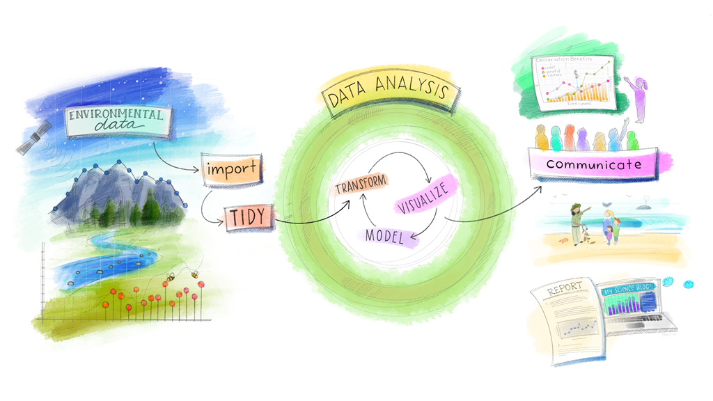
Figure 3.1: The Workflow Revisited. (Artwork by Alison Horst)

Just as in house building, a solid foundation is one of the most important investments you can make in your workflow. I’m fairly certain that you’ve all worked with messy data before but what is tidy data?

3.1 Untidy Data

3.1.1 Toy Data: lynx

Let’s have a quick look at the lynx dataset in R, which records the numbers of lynx trapped in the Mackenzie River District of Canada over time.

# Import the dataset into your working environment
data(lynx)

# View the data
View(lynx)

It seems that the lynx data consists of a vector of values.
In our Environment pane, we can see that there are 114 values, described as a “Time-Series … from 1821 to 1934.”
OK - let’s try and visualise the data with a simple plot using base R:

plot(lynx)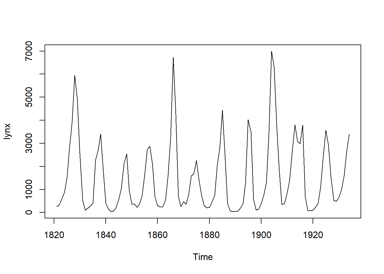

Great! Now let’s try to plot the same graph in using ggplot.

ggplot(
  data = lynx
) +
  geom_line(
    mapping = aes(
      y = ...,
      x = ...
    )
  )

Hmmm… we need to supply a mapping to either ggplot or geom_line, but there are no columns in the lynx data for us to reference by name. Maybe we can just reference the vector of values directly?

# Load ggplot2 into R (and other Tidyverse packages)
library(tidyverse)

# Plot the lynx data
ggplot(
  data = lynx
) +
  geom_line(
    mapping = aes(
      y = lynx # Let's try this because we have no other option
    )
  )

## Error: `data` must be a data frame, or other object coercible by `fortify()`, not an S3 object with class ts

Oops. The error message tells us that our data must be a “data frame,” not a “ts” (time-series). In our first graph, the plot function worked easily, we clearly cannot use ggplot2 on a single vector of values.

Why not?
When we have only a vector of data, we cannot supply the ggplot function with all of the arguments necessary for it to construct the ggplot object. The plot function was coded using a more relaxed expectation of the data that can be supplied. This means that the plot function will nearly always produce a plot if you only supply it with a data argument.

You can test this out for yourself by comparing the lynx plot above with the plot produced if you run this code:

# Load the iris data
data(iris)

# Visualise the data
plot(iris)

Why do you think plot does this? (Hint: Think about the structure of the iris data.)

The trouble with the lynx data is that it is not ‘tidy.’

3.2 What is ‘Tidy Data?’

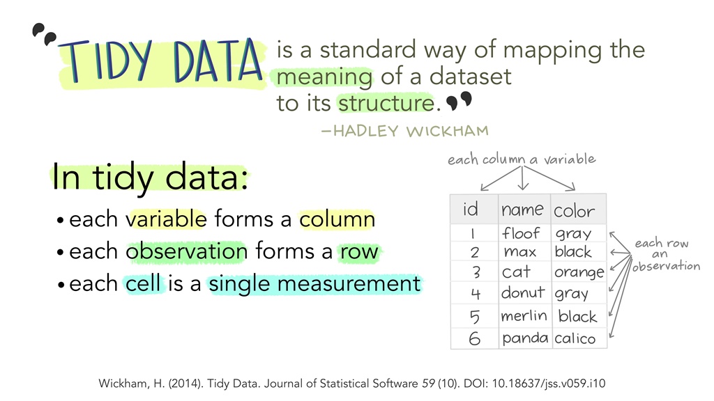
Figure 3.2: Illustration by Alison Horst

Working with tidy data is the principle underlying all the R packages in the ‘Tidyverse’ - such as ggplot2. This is not completely surprising given that ‘tidy’ is the first part of the name, but why is it so useful?

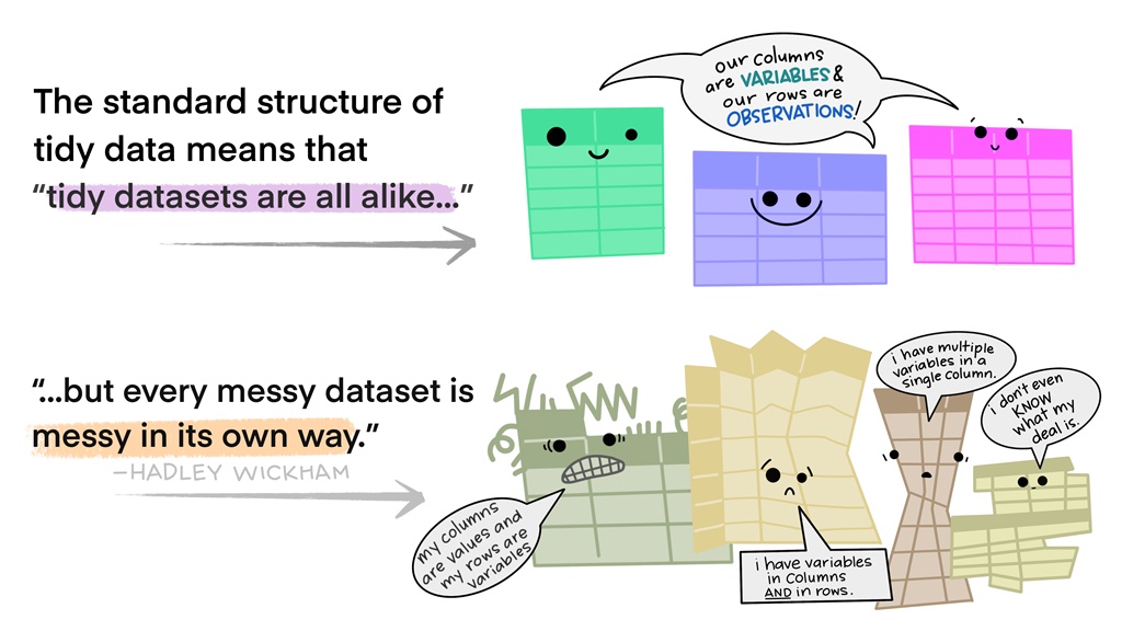
Figure 3.3: Illustration by Alison Horst

The first part of the answer is that the rules produce data in a consistent structure and format for our other functions to work on. And the second reason is because R is a vectorised coding language. Putting both of the above reasons together allowed Hadley Wickham and the Tidyverse team to create the dplyr package.

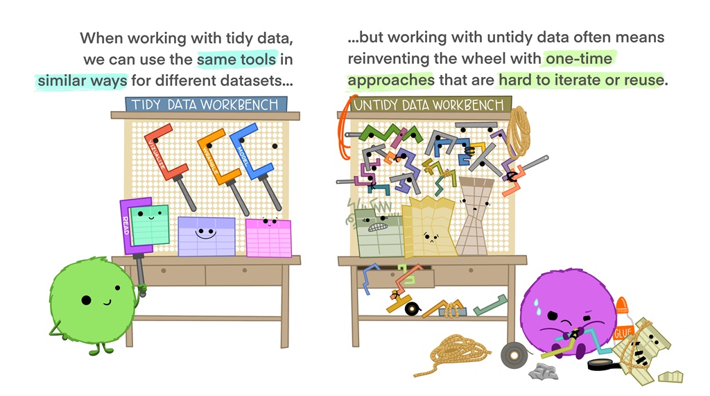
Figure 3.4: Illustration by Alison Horst

Compare the lynx and iris data.

Which one of the two datasets is ‘tidy?’
What would make the ‘untidy’ dataset into a ‘tidy’ one?

3.2.1 The `tibble`

R can import and store data in multiple forms: vectors, lists, data frames and more. When you import data using one of the functions in the Tidyverse e.g., read_csv , the data that you import will be stored as a tibble. In this course you do not need to worry about the finer details but I do want you to know that a tibble is basically a data frame, with some differences in how it is printed to the console.

If you run the code below, you will see a printout of helpful information printed in your Console pane.

library(here)
reptiles <- read_csv(here("data/reptiles.csv"))
head(reptiles)

The Console printout shows you that:

the reptiles object is a tibble,
the number of rows/observations (443),
the number of columns/variables (10),
the variable names e.g., date and species,
the class of each variable e.g., chr = character, dbl = numeric,
the first ten rows/observations in the reptiles object.

Classes are important to understand because many functions in R are built around the class of the data that they expect to operate on. Essentially what this means is that:

# This code WILL work:
data <- c(1, 2, 3, 4, 5)
sum(data)

## [1] 15

# This WILL NOT work
data2 <- c("a", "b", "c")
sum(data2)

## Error in sum(data2): invalid 'type' (character) of argument

If you look at your Environment pane, you will see that data has num (numeric) next to the vector of numbers, while data2 has chr (character) next to its vector of letters. The error message that you get from the sum(data2) code tells you that a character vector is the wrong type of data for the sum function. Giving the wrong type or class of data to a function is a very common source of errors as you begin learning R. The class of a variable is so important that the Tidyverse contains packages that deal with just one type of data:

stringr works with character variables,
forcats works with factor variables,
lubridate works with date variables.

3.3 Package: dplyr

dplyr is one of the most useful packages you can learn to use in R.

Learning to manipulate data frames to complete your analysis or visualisation tasks takes time, patience, and a good tool kit. This is where dplyr comes in because it provides us with the functions that accomplish all of the typical data manipulations we may require across a very wide range of situations.

The main functions in dplyr are all named after English verbs that describe their purpose. The most commonly used ones are:

Change columns/variables:

mutate() adds new variables that are functions of existing variables
select() picks variables based on their names
rename() changes the names of variables

Change rows/observations:

filter() picks cases based on their values
arrange() changes the ordering of the rows

Groups of rows/observations:

group_by creates groups of observations within the tibble (usually for analysis)
summarise() reduces multiple values down to a single summary

3.3.1 `dplyr` in Action

Let’s do some data manipulation (also known as ‘wrangling’) using dplyr!

dplyr should already be loaded because we have loaded the Tidyverse earlier but we can ensure it is loaded again (Note: it does not break anything in R if you try to load a package that has been loaded already).

library(dplyr)

3.3.1.1 Toy Data: msleep

The msleep data set is included in the Tidyverse and is available for us to import after we have loaded the packages into R. It contains information about the sleep habits of 83 mammal species as well as their conservation status, brain weight and body weight.

# Add the msleep data to your R workspace
data(msleep)

# Open the data to inspect it
View(msleep)

Does the msleep data look tidy?

RStudio Tip: In your Environment pane, you can also click on the small drop-down icon next to msleep. This will also show you a helpful summary of the data it contains (including the class of each variable).

3.3.1.2 select()

Lets select the name of each species and the sleep_total variable.

# Select name and sleep_total columns
select(
  msleep,
  sleep_total,
  name
)

Congratulations! You’ve just run your first dplyr function! Let’s inspect what the select function did.

In your Console, you will see that we have dropped all columns/variables except the two that we specified. Note that they also appear in the order we specified them and not in the order that they appear in the msleep object.

Data tidying/manipulation usually involves many steps before we get the data into the state we want. Writing multiple dplyr functions and assigning each output to a new variable becomes long-winded and can be hard to keep track of in your head.

To show you how a sequence of functions can be applied succinctly, I need to now introduce you to one of the signature features of the Tidyverse coding style - the pipe operator.

3.3.1.3 %>% (the pipe)

As you continue to use R, you will see code that looks like this:

msleep %>%
  select(
    sleep_total,
    name
  )

The way this code works is that the %>% operator passes the msleep object as the first argument to the select function. The reason this is useful for us, is because it makes our code human-readable, while ensuring that the code still runs. Learning to use the pipe (%>%) operator is the way to get the most out of the dplyr package.

For the rest of this session, I will use the pipe in the code demonstrations.

3.3.1.4 mutate()

Try this code:

msleep %>%
  mutate(daily_sleep_perc = sleep_total / 24 * 100)

What is different about the printout?

The mutate function allows us to create new variables without modifying any existing variable in our data.

3.3.1.5 rename()

Let’s rename the vore column/variable to diet and the conservation variable to iucn_status.

msleep %>%
  rename(
    diet = vore,
    iucn_status = conservation
  )

Note that we have to specify the name change in the following order: new_name = old_name.

So far we have used functions that manipulate the columns/variables. Now let’s look at the functions that manipulate the rows/observations.

3.3.1.6 filter()

If we are only interested in the sleep data for the omnivores, we can use the following code to remove all carnivore and herbivore observations:

msleep %>%
  filter(
    vore == "omni"
  )

This function is slightly more complicated because we need to use the == operator, which means that we are only interested in cases where the value in vore matches the character string we have supplied i.e., “omni.” If you use only a single =, you will get a helpful error message asking you if perhaps you intended to have used ==.

(Code Tip: For those of you with more experience with R, I encourage you to read about the %in% operator if you haven’t encountered it before. It has more reliable performance than == in some not-uncommon cases.)

3.3.1.7 arrange()

Sometimes we may need to print data as a table in an appendix to a research article or for another reason. If the order of the rows/observations does not match our desired order, we can use arrange to change them.

# Arrange observations in alphabetical order by `name`
msleep %>%
  arrange(name)

# Arrange observations in reverse alphabetical order by name
msleep %>%
  arrange(desc(name))

You will not often need to use arrange but if you do, I advise you to make it the last function you call. I have learned from experience that if you perform operations on the data after arranging the rows, the order can be re-randomised.

arrange is a useful compliment to the group_by function. Let’s look at how it works now.

So far we have looked at functions that can select variables, add new variables, reduce the number of columns in the data frame, reduce the number of rows in the data frame, or modify the order of the observations. The next two functions are useful when we want to perform analysis on our data.

3.3.1.8 group_by()

There are often cases where we are interested in analysing the data for a group of observations.

msleep %>%
  group_by(conservation)

What difference do you see in the printout in your Console?

It can be hard to spot, but there is now a label that reads Groups: conservation [7] at the top of the printout.

3.3.1.9 summarise()

If we want to calculate the mean of sleep_total we can use the following code:

msleep %>%
  summarise(mean_sleep = mean(sleep_total))

What you will notice is that the data frame is gone, and only a single variable remains - called mean_sleep. So let’s look at what the code did.

Within the summarise function, we specified a new variable name (mean_sleep) and then calculated the mean hours of total sleep across all 83 species in our data. The result is a single value - the mean.

Now try this code:

msleep %>%
  summarise(
    mean_sleep = mean(sleep_total),
    min_sleep = min(sleep_total), 
    max_sleep = max(sleep_total)
  )

In this case, we now see the additional variables min_sleep and max_sleep which also contain a single value.

Now, let’s look at what happens when we use the group_by function before running the same summarise code.

msleep %>%
  # We group the observations by their diet i.e. the `vore` variable
  group_by(vore) %>%
  # Now we calculate the mean, min and max values for the sleep_total
  summarise(
    mean_sleep = mean(sleep_total),
    min_sleep = min(sleep_total), 
    max_sleep = max(sleep_total)
  )

Instead of just a single variable, we see that the new data frame consists of a calculation of the mean, maximum and minimum total hours of sleep for each diet group - carni, herbi, insecti, omni, and NA.

I want to show you these two functions from dplyr because in some cases you may find that it is easier to modify your data before you use ggplot2 to visualise it.

3.3.1.10 Example: Putting `dplyr` and `ggplot2` together

In this example, we will be modifying the msleep tibble and then passing it into ggplot for plotting with a geom called geom_pointrange.

# Create a new data frame from the msleep data
# We will assign it to a new object called 'summary_data'
summary_data <- msleep %>%
  group_by(vore) %>%
  summarise(
    mean_sleep = mean(sleep_total),
    min_sleep = min(sleep_total),
    max_sleep = max(sleep_total)
  )

Now we can use the new data frame we created as the basis for our visualisation.

# Now we can PIPE the 'summary_data' into ggplot
summary_data %>%
  ggplot(
    aes(
      x = vore,
      y = mean_sleep,
      ymin = min_sleep,
      ymax = max_sleep
    )
  ) +    # but REMEMBER to use the '+' to add ggplot functions!
  geom_pointrange()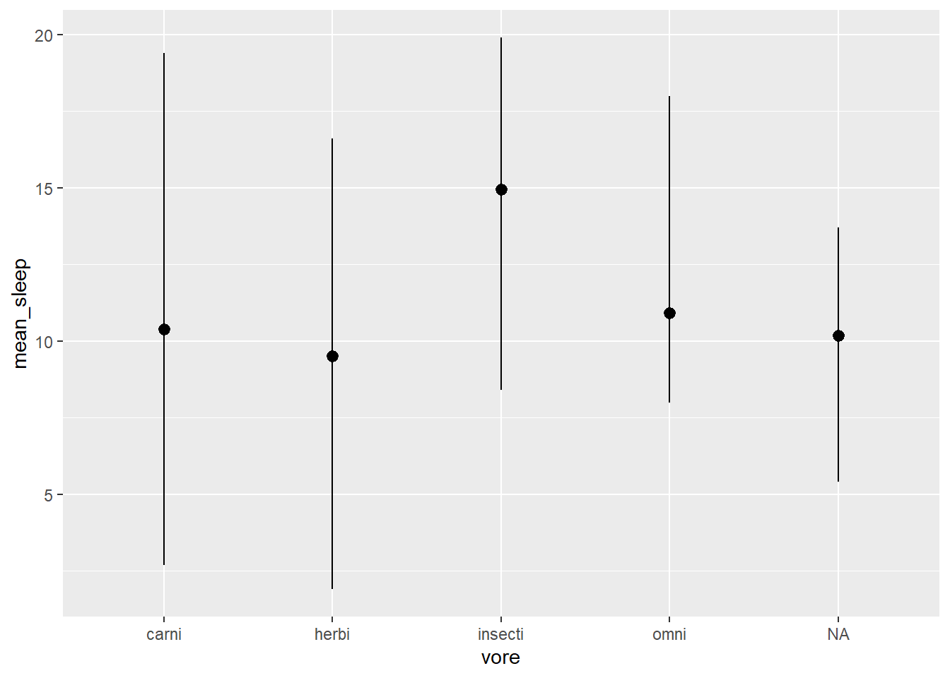

3.3.2 Laura’s Boxplot

During the session, Laura asked a question about whether it is possible to create a boxplot similar to the plot above, without modifying the msleep data using dplyr first.

Yes it is. Here is the code to do that:

msleep %>% 
  ggplot() +
  geom_boxplot(
    aes(
      x = vore,
      y = sleep_total
    )
  )

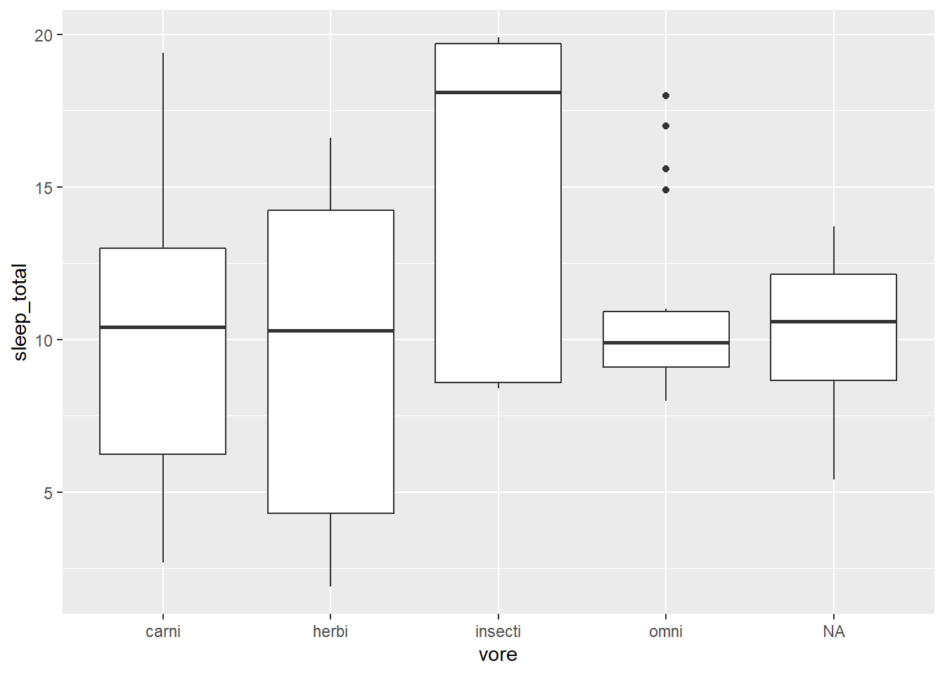
The reason that we can do this is because the default for the stat argument in geom_boxplot is “boxplot.” The default stat for geom_pointrange is “identity” (which means to plot the values as they are provided - no modification).

What this means is that stat in geom_boxplot does the work we did using dplyr in our plot using geom_pointrange.

As with all things Tidyverse, there are many ways to get the job done.

3.4 Exercises

Use a dplyr function to produce a data frame of just the name, vore, brainwt and bodywt variables. (Bonus points if you use the %>% operator!)
Use the mutate function to calculate the percentage of each day that each species is awake. (Assign your calculation to a variable called awake_perc).
Rename the name variable to common_name.
Which species has the highest total number of hours sleep in our data set? (Hint: You can reorder the data appropriately to find the answer.)
Using ggplot2 create a scatter plot of bodywt vs sleep_total, and colour the points according to diet.
Try to create a visualisation of any part of the msleep data that you are interested in. Use the skills and code snippets from the last two sessions to do so.