13.1 Regressão linear no R

Carregar pacotes

library(readxl)
library(ggplot2)

Carregar dados:

estudomg <- read_excel("/Users/eugeniaviana/Documents/Documents/Eugenia/Sociologia/Disciplinas/Analise de dados/Regressão Linear/estudomg.xlsx")

Em seguida, montamos o modelo de regressão com a função lm()

reg<-lm(estudomg$Ensmedio ~ estudomg$Rendamedia)

summary(reg)

## 
## Call:
## lm(formula = estudomg$Ensmedio ~ estudomg$Rendamedia)
## 
## Residuals:
##      Min       1Q   Median       3Q      Max 
## -24.6468  -2.9908  -0.2523   2.7899  20.1145 
## 
## Coefficients:
##                      Estimate Std. Error t value Pr(>|t|)    
## (Intercept)         5.3666662  0.5017685   10.70   <2e-16 ***
## estudomg$Rendamedia 0.0303539  0.0009646   31.47   <2e-16 ***
## ---
## Signif. codes:  0 '***' 0.001 '**' 0.01 '*' 0.05 '.' 0.1 ' ' 1
## 
## Residual standard error: 4.873 on 851 degrees of freedom
## Multiple R-squared:  0.5378, Adjusted R-squared:  0.5373 
## F-statistic: 990.3 on 1 and 851 DF,  p-value: < 2.2e-16

Por fim, montamos o gráfico de regressão no ggplot

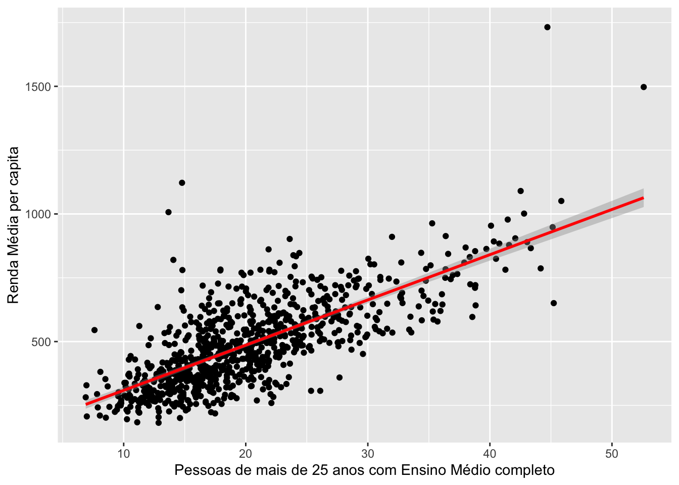
ggplot(estudomg, aes(x = Ensmedio, y = Rendamedia)) + 
  geom_point() +
  stat_smooth(method = "lm", col = "red")+
  xlab("Pessoas de mais de 25 anos com Ensino Médio completo")+
  ylab("Renda Média per capita")

## `geom_smooth()` using formula = 'y ~ x'