26 Simulation and Prediction
26.1 Predicting Outcomes of Sporting Events
This chapter will lay out a strategy to predict the results of the NCAA Division I Women’s Volleyball tournament which was held over three weekends in December, 2019, using match data from the 2019 regular season and conference tournaments as predictors. The tournament had 63 matches in a full bracket to reduce 64 teams down to a single bracket. The top 16 teams were seeded from #1 Baylor to #16 Purdue. Each of these teams hosted the first and second rounds of the tournament for four teams during the first weekend. The sixteen winners in the second round then went to host sites (as it was, the top four seeded teams were wmong the winners and hosted again) four the third and fourth rounds. The four champions advanced to Pittsburgh, Pennsylvania for the national semi-finals and the finals match.
26.2 Model Recap
The model we used assumes that each team has an overall strength factor \(\theta\) (an average team has \(\theta = 0\)) and that the difference \(\Delta_{ij} = \theta_i - \theta_j\) governs the probability that each team wins a point, with the probability that team \(i\) wins equal to the inverse logistic formula \[ \mathsf{P}(\Delta_{ij}) = \frac{1}{1 + \exp(-\Delta_{ij})} \] In match \(k\), let \(i(k)\) be the index of the first team and \(j(k)\) be the index of the second team and let \(x_k\) and \(y_k\) be the total points scored by the first and and second teams, respectively in the match. The likelihood as a function of the vector \(\theta = (\theta_1,\ldots,\theta_m)\) if there are \(m\) total teams and \(n\) total matches is then \[ L(\theta) = \prod_{k=1}^n \mathsf{P}(\Delta_{i(k)j(k)})^{x_k}(1 - \mathsf{P}(\Delta_{i(k)j(k)}))^{y_k} \] The individual values of \(\theta_i\) are only identifiable up to an additive constant in this model as \(\theta_i - \theta_j = (\theta_i + c) - (\theta_j + c)\) for any \(c\). Therefore, we assume that the sum (and mean) of the \(\theta_i\) values is equal to zero. \[ \sum_{i=1}^m \theta_i = 0 \] With this model, we can then use a numerical estimation routine to find maximum likelihood estimates of \(\theta\) from the 2019 season data.
26.3 Estimation of Volleyball Model
This block of code reads in the match data.
From this, it calculates the total number of points won by each team per match and identifies a team index for each team.
It creates data frames vb with the summarized match data
and teams with the team names and indices.
The variable home is 1 when team2 is the home team.
## Read the data
vb_season = read_csv("data/vb-division1-2019-all-matches-corrected.csv")

## repair a missing winner variable
vb_season %>% rowwise() %>% mutate(max = max(sets_1,sets_2)) %>% filter(max != 3)
# A tibble: 1 × 23
# Rowwise:
index date team1 conference1 team2 conference2 site s1_1 s1_2 s1_3
<dbl> <date> <chr> <chr> <chr> <chr> <chr> <dbl> <dbl> <dbl>
1 1972 2019-09-24 Saint … MAAC Lafa… Patriot <NA> 25 21 17
# ℹ 13 more variables: s1_4 <dbl>, s1_5 <dbl>, sets_1 <dbl>, s2_1 <dbl>,
# s2_2 <dbl>, s2_3 <dbl>, s2_4 <dbl>, s2_5 <dbl>, sets_2 <dbl>, winner <chr>,
# loser <chr>, attendance <dbl>, max <dbl>vb_season$sets_1[1972] = 2
vb_season$sets_2[1972] = 3
vb_season$winner[1972] = vb_season$team2[1972]
vb_season$loser[1972] = vb_season$team1[1972]
## Summarize to find total points
vb = vb_season %>%
select(-matches("sets."), -attendance, -date) %>%
rowwise() %>%
mutate(points1 = sum(c_across(matches("s1_[1-5]")), na.rm = TRUE),
points2 = sum(c_across(matches("s2_[1-5]")), na.rm = TRUE)) %>%
ungroup() %>%
mutate(home = as.integer(is.na(site))) %>%
select(-matches("s[12]_[1-5]")) %>%
rename(match_index = index)
## Find teams
teams = vb %>%
count(team1,conference1) %>%
mutate(index = row_number()) %>%
select(index,team1, conference1) %>%
rename(team = team1,
conference = conference1) %>%
left_join( vb %>% count(winner), by = c("team" = "winner") ) %>%
rename(wins = n) %>%
left_join( vb %>% count(loser), by = c("team" = "loser") ) %>%
rename(losses = n) %>%
mutate(wins = case_when(
is.na(wins) ~ 0L,
TRUE ~ wins),
losses = case_when(
is.na(losses) ~ 0L,
TRUE ~ losses))
## Add index variables
vb = vb %>%
left_join(teams %>% select(team,index), by = c("team1" = "team")) %>%
rename(index1 = index) %>%
left_join(teams %>% select(team,index), by = c("team2" = "team")) %>%
rename(index2 = index)26.3.1 Maximum Likelihood Estimate of \(\theta\)
We use optim() to calculate the maximum likelihood estimate of \(\theta\).
An initial \(\theta\) has all values equal to zero.
We maximize the log-likelihood allowing for all \(\theta_i\) except the last
where \(i=m\), setting \(\theta_m\) to be the negative sum of the other \(\theta_i\).
At the end of the calculation, we add the estimated \(\theta\) values to the team data frame.
mle_theta = function(matches, teams)
{
  n_teams = nrow(teams)
  theta_0 = rep(0,n_teams-1)

  inv_logistic = function(x) { return ( 1/(1 + exp(-x)) ) }

  calc_logl = function(theta, df)
  {
    delta = theta[df$index1] - theta[df$index2]
    p = inv_logistic(delta)
    return ( sum( df$points1*log(p) + df$points2*log(1-p)) )
  }

  f = function(theta,df)
  {
    theta = c(theta,-sum(theta))
    return ( calc_logl(theta,df) )
  }

  out = optim(theta_0, f, method="BFGS",
              control=list(fnscale=-1), df=matches)

  return ( out )
}

mle_out = mle_theta(vb, teams)

## convergence indicated if 0
mle_out$convergence
[1] 026.3.2 Exploration
Examine the distribution of \(\theta\) values among the teams. The mean is zero (by design). The shape is more or less bell-shaped. The poor teams are a bit more extreme than the strong teams.
ggplot(teams, aes(x=theta)) +
  geom_histogram(boundary=0, binwidth=0.04, fill="firebrick", color="black")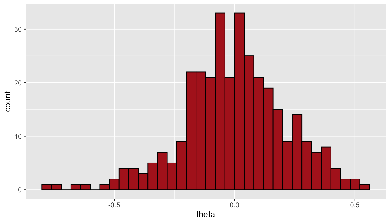
Examine the distribution of \(\theta\) by conference. The conferences are ordered by mean value of \(\theta\) within the conference. Here are some observations:
- The strongest overall conference is the Pac-12 and the Pac-12 has the best team (Stanford).
- The second best team is the best team in the Big Ten (Wisconsin).
- The Big Ten is more variable than the Pac-12.
- The top quarter of the Big Ten are stronger than the second best Pac-12 team
- The bottom of the Big Ten is much weaker than the bottom of the Pac-12.
- The bottom half of the Big 12 is much weaker than the those of other top conferences.
- The top few teams in the Big 12 faced much weaker competition for much of their schedule as compared to the top teams in the Big Ten and the Pac-12.
- A few conferences, such as the Mountain West and Conference USA had a single team that was much stronger than the rest of the conference.
teams %>%
  mutate(conference = reorder(conference,theta)) %>%
ggplot(aes(x=conference, y=theta)) +
  geom_boxplot(fill = "firebrick") +
  coord_flip()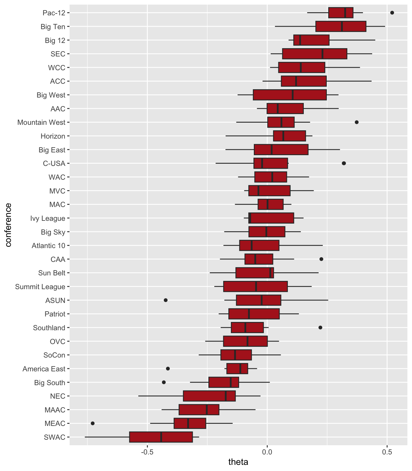
Let’s examine the top 10 teams as estimated by the data.
# A tibble: 10 × 7
   index team       conference  wins losses theta  rank
   <int> <chr>      <chr>      <int>  <int> <dbl> <int>
 1   263 Stanford   Pac-12        24      4 0.521     1
 2   326 Wisconsin  Big Ten       22      6 0.492     2
 3   178 Nebraska   Big Ten       25      4 0.482     3
 4   211 Penn St.   Big Ten       24      5 0.474     4
 5   272 Texas      Big 12        21      3 0.451     5
 6   131 Kentucky   SEC           23      6 0.438     6
 7   213 Pittsburgh ACC           29      1 0.435     7
 8    22 Baylor     Big 12        25      1 0.434     8
 9   163 Minnesota  Big Ten       23      5 0.429     9
10   315 Washington Pac-12        24      6 0.399    10
Stanford is rated as the best team by a wide margin, even though they had four regular season losses. Wisconsin is rated as the second strongest team, ahead of the other three Big 10 teams in the top 10.
However, the NCAA selection committee seeded the teams differently. The NCAA seeded Baylor #1 and Texas #2 from the Big 12 conference, where we have them ranked 8th and 5th strongest.
ncaa = read_csv("data/vb-division1-2019-ncaa-tourney.csv")

ncaa_teams = ncaa %>%
  select(team1, team2) %>%
  pivot_longer(everything(), names_to = "pos", values_to = "team") %>%
  select(-pos) %>%
  distinct() %>%
  mutate(seed = parse_number(team)) %>%
  mutate(team = case_when(
    is.na(seed) ~ team,
    TRUE ~ str_replace(team,"^[[:digit:] ]+",""))) %>%
  left_join(teams) %>%
  arrange(seed, conference, team)

ncaa_teams %>%
  head(n=16)
# A tibble: 16 × 8
team seed index conference wins losses theta rank
<chr> <dbl> <int> <chr> <int> <int> <dbl> <int>
1 Baylor 1 22 Big 12 25 1 0.434 8
2 Texas 2 272 Big 12 21 3 0.451 5
3 Stanford 3 263 Pac-12 24 4 0.521 1
4 Wisconsin 4 326 Big Ten 22 6 0.492 2
5 Nebraska 5 178 Big Ten 25 4 0.482 3
6 Pittsburgh 6 213 ACC 29 1 0.435 7
7 Minnesota 7 163 Big Ten 23 5 0.429 9
8 Washington 8 315 Pac-12 24 6 0.399 10
9 Kentucky 9 131 SEC 23 6 0.438 6
10 Florida 10 84 SEC 25 4 0.388 12
11 Penn St. 11 211 Big Ten 24 5 0.474 4
12 Hawaii 12 105 Big West 24 3 0.297 29
13 Texas A&M 13 273 SEC 20 7 0.336 21
14 BYU 14 20 WCC 25 4 0.379 14
15 Western Ky. 15 321 C-USA 31 1 0.320 24
16 Purdue 16 220 Big Ten 22 7 0.360 17# A tibble: 5 × 8
team seed index conference wins losses theta rank
<chr> <dbl> <int> <chr> <int> <int> <dbl> <int>
1 Utah NA 306 Pac-12 22 9 0.392 11
2 San Diego NA 240 WCC 24 5 0.387 13
3 Colorado St. NA 56 Mountain West 29 1 0.373 15
4 Illinois NA 115 Big Ten 16 13 0.360 16
5 UCLA NA 289 Pac-12 18 11 0.346 19Note that our ranking method ignores the won lost record of teams, does not explicitly use conference, treats games equally from early in the season to late, and does not consider rankings by people or the press. The selection committee does. Specifically, the number one seed Baylor had only one loss (and had more wins than shown here counting non-division I opponents), did beat Wisconsin head-to-head early in the year, and was champion in a power conference. They earned the number 1 seed, even if we think (and calculate under a model) that Wisconsin is a stronger team. Let’s see how our estimates may be used for prediction in the tournament.
26.4 Predicting the Tournament
The model estimates the probability that each team wins a point in a match between two opponents, but does not directly allow us to calculate the probability that a team wins a set or a match. We use simulation to estimate these probabilities. Specifically, we consider a sequence of independent coin tosses for the estimated win probability and follow the rules of scoring volleyball until one team has one the match. We repeat a large number of times for each potential match. Rather than predicting the entire tournament, let’s make predictions prior to each of Wisconsin’s matches. The code for the predictions is in the following large code block.
inv_logistic = function(x) { return ( 1/(1 + exp(-x)) )}

sim_set = function(delta,target)
{
  p = inv_logistic(delta)
  points = c(0,0)
  repeat
  {
    pt = rbinom(1,1,p)
    if ( pt == 1 )
      points[1] = points[1] + 1
    else
      points[2] = points[2] + 1
    if ( max(points) >= target && abs(diff(points)) >= 2 )
      break
  }
  return ( points )
}

sim_match = function(delta)
{
  tab = matrix(NA,2,5)
  sets = c(0,0)
  index = 1
  repeat
  {
    if ( sum(sets) < 4 )
      result = sim_set(delta,25)
    else
      result = sim_set(delta,15)
    if ( result[1] > result[2] )
      sets[1] = sets[1] + 1
    else
      sets[2] = sets[2] + 1
    tab[,index] = result
    index = index + 1
    if ( max(sets == 3) )
      break
  }
  return ( tab )
}

extract_one_match = function(matches, name1, name2)
{
  out = matches %>%
    filter(team1 == name1 & team2 == name2) %>%
    select(matches("s._.")) %>%
    pivot_longer(everything(), names_to = "team_set", values_to = "points") %>%
    separate(team_set, into = c("team","set")) %>%
    pivot_wider(names_from = set, values_from = points) %>%
    select(-team) %>%
    as.matrix()
  return ( out )
}

show_one_match = function(m, name1, name2)
{
  dat = tibble(team = c(name1, name2)) %>%
    bind_cols(as_tibble(m), .name_repair = "minimal")

  return ( dat )
}

sim_many_matches = function(B, teams, team1, team2)
{
  result = rep(0,B)
  team1_pts = rep(0,B)
  team2_pts = rep(0,B)

  theta1 = teams %>%
    filter(team == team1) %>%
    pull(theta)

  theta2 = teams %>%
    filter(team == team2) %>%
    pull(theta)

  delta = theta1 - theta2

  for ( i in 1:B)
  {
    m = sim_match(delta)
    result[i] = ( sum(m[1,] > m[2,], na.rm=TRUE) == 3 )
    team1_pts = sum(m[1,], na.rm = TRUE)
    team2_pts = sum(m[2,], na.rm = TRUE)
  }

  win1 = round(mean(100*mean(result)), 1)
  win2 = 100 - win1
  p1 = round(inv_logistic(theta1 - theta2),3)
  p2 = 1 - p1

  cat(team1,"versus",team2,"\n")
  cat("win %:", team1, "=", win1, ", ", team2, "=", win2, "\n")
  cat("point probability:", team1, "=", p1, ", ", team2, "=", p2, "\n")
  return(invisible())
}

get_delta = function(teams, name1, name2)
{
  theta1 = teams %>%
    filter(team == name1) %>%
    pull(theta)

  theta2 = teams %>%
    filter(team == name2) %>%
    pull(theta)

  return(theta1 - theta2)
}
26.4.1 The simulations
26.4.1.1 Wisconsin versus Illinois St.
On December 6, 2019, Wisconsin played Illinois State in Madison, Wisconsin. The Badgers were heavily favored and won.
name1 = "Illinois St."

name2 = "Wisconsin"

delta = get_delta(ncaa_teams, name1, name2)

## Real Match
show_one_match( extract_one_match(ncaa, name1, "4 Wisconsin"),
                name1, name2 )
# A tibble: 2 × 6
team `1` `2` `3` `4` `5`
<chr> <dbl> <dbl> <dbl> <dbl> <dbl>
1 Illinois St. 13 14 24 NA NA
2 Wisconsin 25 25 26 NA NAWarning: The `x` argument of
`as_tibble.matrix()` must have
unique column names if
`.name_repair` is omitted as of
tibble 2.0.0.
ℹ Using compatibility
`.name_repair`.
This warning is displayed once
every 8 hours.
Call
`lifecycle::last_lifecycle_warnings()`
to see where this warning was
generated.# A tibble: 2 × 6
team V1 V2 V3 V4 V5
<chr> <dbl> <dbl> <dbl> <dbl> <dbl>
1 Illinois St. 12 24 19 NA NA
2 Wisconsin 25 26 25 NA NAIllinois St. versus Wisconsin
win %: Illinois St. = 1.9 , Wisconsin = 98.1
point probability: Illinois St. = 0.421 , Wisconsin = 0.579 26.4.1.2 Wisconsin versus UCLA
On December 7, 2019, Wisconsin played Pac-12 team UCLA in Madison, Wisconsin. The Badgers were big favorites and won.
name1 = "UCLA"
name2 = "Wisconsin"

delta = get_delta(ncaa_teams, name1, name2)

## Real Match
show_one_match( extract_one_match(ncaa, name1, "4 Wisconsin"),
                name1, name2 )
# A tibble: 2 × 6
team `1` `2` `3` `4` `5`
<chr> <dbl> <dbl> <dbl> <dbl> <dbl>
1 UCLA 18 21 14 NA NA
2 Wisconsin 25 25 25 NA NA# A tibble: 2 × 6
team V1 V2 V3 V4 V5
<chr> <dbl> <dbl> <dbl> <dbl> <dbl>
1 UCLA 20 17 25 25 7
2 Wisconsin 25 25 18 23 15UCLA versus Wisconsin
win %: UCLA = 16.7 , Wisconsin = 83.3
point probability: UCLA = 0.464 , Wisconsin = 0.536 26.4.1.3 Wisconsin versus Texas A&M
On December 13, 2019, Wisconsin played #13 Texas A&M in Madison, Wisconsin. The Badgers were big favorites and won.
name1 = "Texas A&M"
name2 = "Wisconsin"

delta = get_delta(ncaa_teams, name1, name2)

## Real Match
show_one_match( extract_one_match(ncaa, "13 Texas A&M", "4 Wisconsin"),
                name1, name2 )
# A tibble: 2 × 6
team `1` `2` `3` `4` `5`
<chr> <dbl> <dbl> <dbl> <dbl> <dbl>
1 Texas A&M 20 17 23 NA NA
2 Wisconsin 25 25 25 NA NA# A tibble: 2 × 6
team V1 V2 V3 V4 V5
<chr> <dbl> <dbl> <dbl> <dbl> <dbl>
1 Texas A&M 25 20 22 NA NA
2 Wisconsin 27 25 25 NA NATexas A&M versus Wisconsin
win %: Texas A&M = 15.9 , Wisconsin = 84.1
point probability: Texas A&M = 0.461 , Wisconsin = 0.539 26.4.1.4 Wisconsin versus Nebraska
On December 14, 2019, Wisconsin played #5 Nebraska in Madison, Wisconsin. Both teams were very evenly matched (a model that takes home court into account favored the Badgers a bit more). The Badgers remained victorious and advanced to the Final Four!
name1 = "Nebraska"
name2 = "Wisconsin"

delta = get_delta(ncaa_teams, name1, name2)

## Real Match
show_one_match( extract_one_match(ncaa, "5 Nebraska", "4 Wisconsin"),
                name1, name2 )
# A tibble: 2 × 6
team `1` `2` `3` `4` `5`
<chr> <dbl> <dbl> <dbl> <dbl> <dbl>
1 Nebraska 18 22 19 NA NA
2 Wisconsin 25 25 25 NA NA# A tibble: 2 × 6
team V1 V2 V3 V4 V5
<chr> <dbl> <dbl> <dbl> <dbl> <dbl>
1 Nebraska 13 25 12 27 15
2 Wisconsin 25 22 25 25 5Nebraska versus Wisconsin
win %: Nebraska = 47.2 , Wisconsin = 52.8
point probability: Nebraska = 0.498 , Wisconsin = 0.502 26.4.1.5 Wisconsin versus Baylor
In the national semifinals, Wisconsin faced #1 Baylor in Pittsburgh, Pennsylvania. The model made the Badgers favorites, even if the seeding and won-loss record did not. The Badgers won in four sets!
name1 = "Wisconsin"
name2 = "Baylor"

delta = get_delta(ncaa_teams, name1, name2)

## Real Match
show_one_match( extract_one_match(ncaa, "4 Wisconsin", "1 Baylor"),
                name1, name2 )
# A tibble: 2 × 6
team `1` `2` `3` `4` `5`
<chr> <dbl> <dbl> <dbl> <dbl> <dbl>
1 Wisconsin 25 25 25 25 NA
2 Baylor 27 21 17 19 NA# A tibble: 2 × 6
team V1 V2 V3 V4 V5
<chr> <dbl> <dbl> <dbl> <dbl> <dbl>
1 Wisconsin 18 25 23 19 NA
2 Baylor 25 19 25 25 NAWisconsin versus Baylor
win %: Wisconsin = 65 , Baylor = 35
point probability: Wisconsin = 0.514 , Baylor = 0.486 26.4.1.6 Wisconsin versus Stanford
The final match pitted #3 Stanford versus #4 Wisconsin. The model said that Stanford was the strongest team and they were favored over the Badgers. UW lost and finished as runners up for the national championship.
name1 = "Wisconsin"
name2 = "Stanford"

delta = get_delta(ncaa_teams, name1, name2)

## Real Match
show_one_match( extract_one_match(ncaa, "4 Wisconsin", "3 Stanford"),
                name1, name2 )
# A tibble: 2 × 6
team `1` `2` `3` `4` `5`
<chr> <dbl> <dbl> <dbl> <dbl> <dbl>
1 Wisconsin 16 17 20 NA NA
2 Stanford 25 25 25 NA NA# A tibble: 2 × 6
team V1 V2 V3 V4 V5
<chr> <dbl> <dbl> <dbl> <dbl> <dbl>
1 Wisconsin 21 20 25 14 NA
2 Stanford 25 25 14 25 NAWisconsin versus Stanford
win %: Wisconsin = 42.5 , Stanford = 57.5
point probability: Wisconsin = 0.493 , Stanford = 0.507