23 Human Sex Ratio Modeling
23.1 Is it a boy or a girl?
When a couple is expecting a new child, there is frequently great interest in knowing what the sex of the child will be. Traditional baby showers often included games some believed could reliably predict the sex of the coming baby. When sharing the news of a new baby, after asking about the health of the newborn and mother (and maybe the father too), the pieces of information the new parents are expected often to share are the name, sex, and weight. For the past several decades, the use of ultrasound during routine prenatal care has given parents the option to learn the sex of their baby months before it is born. (My wife and I opted to remain ignorant of this piece of information for each of our four children, having a preference for an additional surprise at the birth.) The phenomenon of extravagant “reveal parties” where couples share the sex of the expected child with some spectacular event, often that produces the color blue for a boy or pink for a girl seem to be increasing in popularity, even as some number result in mishap or tragedy when events spin out of control.
In the scientific literature, the ratio of the number of boys per one hundred girls among live births in some population is known as the secondary sex ratio. The primary sex ratio is this value at conception and a tertiary sex ratio refers to the sex ratio at an older age of development. There is a substantial literature on the human secondary sex ratio with interest in changes over time, differences among different populations, and potential associated factors, such as hormone levels at the time of conception, age of the parents, and the timing of conception during the mother’s cycle. Part of the scientific interest stems from the fact that most nations track and publish data annually on the number of live births and the numbers of boys and girls born each year, so there is substantial data available.
23.2 A Note on Gender Identity
We do note that for many people, the sex assigned at birth does not match their own gender identity. Some people identify with the sex opposite to the one assigned at birth and others identify as nonbinary, not belonging to either gender. As a matter of practice, secondary sex identity is based on superficial examination of genitalia of the newborn. Even this is not a perfect measure as there are a small fraction of individuals with sexual organs from both sexes or neither, or those whose sexual organs may develop later in life. Scientific understanding of both sex and gender identity contains much uncertainty. In addition, social norms in the United States are rapidly changing as general awareness increases of the frequency of people whose gender identity does not match their sex assigned at birth and the associated issues of relationships among family, friends and coworkers, public bathroom restrictions, legal relationships, pronoun usage, and more.
Gender identity and how society responds are important and interesting topics, but are not the subject of this chapter which aims to explore models of human secondary sex ratios. In the remainder of this chapter, when we refer to sexual identity as a boy (male) or girl (female), we are referring to the labels which are assigned at birth and are recorded as government statistics, in full recognition that these labels are inaccurate for many people around the world, including, perhaps, some of the readers of this chapter.
23.3 Sex Ratio Data
In this chapter we will refer to four data sets, three of which are well studied in the scientific literature on human sex ratios. Three data sets are from European populations over different time periods in the past 150 years. Each of these data sets records sexes of children in families, totalling millions of children. The fourth data set is modern data with sex ratio summaries by country in the world. Each of the data sets has issues with how the data is collected and shared.
23.3.1 Geissler Data, Saxony
The first data set is a subset from a massive data collection made by Geissler and published in 1889 from church birth records in Saxony (in modern times a region in eastern Germany) during 1876–1885. During this time, each birth certificate was required to contain all of the children in the family. As a consequence, families will appear multiple times in the data set if they had multiple children during this period (as most did), and many births are recorded multiple times (when they happened, and when younger siblings were born). However, all records from a given family size will correspond to separate families. There was some filtering as well as birth certificates for when there were multiple births (twins, triplets, and so on) were excluded.
Previous researchers also made an odd choice which can affect the interpretation of the results. The data we have for each family size actually shows results of the sexes among the first \(k-1\) kids at the time of the birth of the \(k\)th kid. The reason given for this odd choice was to lessen the presumed bias due to the decision to stop having more children based on the sex of the last child. (The researchers thought some families might be more likely to stop having more children if the last child was a boy.) While such biases certainly are real, the decision, however, ignores potential bias from making that same decision being after the birth of the previous child. We will generally ignore this aspect of the data. Furthermore, we will tend to only analyze the data about families of a fixed size to avoid having the same families appear multiple times during the analysis.
The data from this study is in a file with the name geissler.csv.
# A tibble: 6 × 4
   boys girls  size   freq
  <dbl> <dbl> <dbl>  <dbl>
1     0     1     1 108719
2     0     2     2  42860
3     0     3     3  17395
4     0     4     4   7004
5     0     5     5   2839
6     0     6     6   1096
The format of the data is a long data frame with one row for each family size and combination of boys and girls. The variables are:
boys: the number of boys in each family in that row;girls: the number of girls in each family in that row;size: the number of children in each family (boys + girls);freq: the number of families of the given size with that number of boys and girls.
So, for example, there are 108,719 families in the data set where the first child was a girl. (More correctly, there were 108,719 families that had a second child where the first child was a girl. But we will ignore this from now on.) There are also 42,860 families with two children where both are girls. This group will have a large overlap with the 108,719 from the first row. (A family could be included in the second row and not the first if the birth of the first child did not occur during the years of the study.)
We will often examine a subsample of the data set for all families of a given size. Here, for example are families with four children.
# A tibble: 5 × 4
boys girls size freq
<dbl> <dbl> <dbl> <dbl>
1 0 4 4 7004
2 1 3 4 28101
3 2 2 4 44793
4 3 1 4 31611
5 4 0 4 8628We can sum up the number of families and determine the total number of boys and girls in these families. With these summary statistics, we can calculate the observed proportion of boys and the observed sex ratio.
geissler %>%
filter(size == 4) %>%
summarize(families = sum(freq),
boys = sum(boys*freq),
girls = sum(girls*freq)) %>%
mutate(p_boy = boys / (boys+girls),
sex_ratio = 100*boys/girls)# A tibble: 1 × 5
families boys girls p_boy sex_ratio
<dbl> <dbl> <dbl> <dbl> <dbl>
1 120137 247032 233516 0.514 106.- Note that there are 991,958 families.
- To count the number of boys, it was necessary to sum the product of
boysandfreq. There are:- 0 boys among the 7004 families with 0 boys and 4 girls.
- 28,101 boys among the 28,101 families with 1 boy and 3 girls.
- \(2 \times 44,793 = 89,586\) boys among the families with 2 boys and 2 girls.
- \(3 \times 31,611 = 93,833\) boys among the families with 3 boys and 1 girl.
- \(4 \times 8,628 = 34,512\) boys among the families with 4 boys and 0 boys.
A similar calculation is made for the girls.
The proportion of boys in families of size 4 in this data set is \(247,032/(247,032 + 233,516) \doteq 0.514\)
The sex ratio is \(100 \times 247,032/233,516 \doteq 105.8\).
The Geissler data set has data on families from size 1 to 12.
23.3.2 Malinvaud Data, France
A second large data set was collected from families in France from 1946 to 1950. 1 Each family has a mother who had no previous children only single births. In this data set, each child is counted only once and is tabulated according to the number of boys and girls who preceded them in the family.
The data from this study is in a file named french-children.csv. Here are the first few rows of the data set.
# A tibble: 6 × 4
  girls  boys count p_boy
  <dbl> <dbl> <dbl> <dbl>
1     0     0  1499 0.514
2     0     1   552 0.519
3     0     2   163 0.527
4     0     3    45 0.525
5     0     4    13 0.544
6     0     5     4 0.535
The format again is a long data format with these variables:
girlsis the number of previous girls in the family;boysis the number of previous boys in the family;countis the number of children (in 1000s) born with the corresponding number of older children by assigned sex at birth;p_boyis the fraction of children in thecountthat are boys.
The first row tells us that there are 1,499,000 families in the data set (all counts are rounded to the nearest 1000) and that 51.4%, or 770,486 of the first-born children are boys and 48.6%, or 728,514 are girls. The second row indicates that 552,000 families of the 770,486 families who had a first boy had a second child, and of these second children, 51.9% were boys and 48.1% were girls. This data is more informative than the data from Saxony as we can determine for each family composition of previous children, the proportion of families that have another child and if so, the proportion of the sex assigned at birth of these children.
23.3.3 Danish Data
The third data set was collected from all Danish families from 1960 to 1994 with only single births. This data set is even more detailed than the data from France as it has counts based on the sexes of the previous children in order, not only the numbers of boys and girls already in the family. The data summary includes the numbers of male and females born as the first, second, third, fourth, or fifth single birth in their family, broken down by the order of any previous singular births in the family. This data allows us to examine how the genders of previous children affects if a family has another child, and if they do, how the past genders affect the probability that the next child is female or male.
Data is in the file danish-children.csv. Here are the first few rows of the data set.
# A tibble: 10 × 4
   order sex   previous      n
   <dbl> <chr> <chr>     <dbl>
 1     1 F     <NA>     341522
 2     1 M     <NA>     358508
 3     2 F     F        121801
 4     2 M     F        126840
 5     2 F     M        127123
 6     2 M     M        135138
 7     3 F     FF        18770
 8     3 M     FF        19414
 9     3 F     FM        16814
10 3 M FM 18559- The data includes a summary of 1,403,021 children born to 700,030 couples.
- Each row of the data frame has this information:
order: the birth order (from 1 to 5)sex: F (female) or M (male)previous: the pattern of previous female and male single births in the familyn: the number of families with a child of a given sex and birth order
23.3.4 World Sex Ratios
The final data set includes sex ratios for countries around the world estimated by the CIA for 2020 and also has population data. This data is in the file world-sex-ratios.csv.
# A tibble: 6 × 9
  Country    birth ages_0_14 ages_15_24 ages_25_54 ages_55_64 ages_over_65 Total
  <chr>      <dbl>     <dbl>      <dbl>      <dbl>      <dbl>        <dbl> <dbl>
1 Afghanist…  1.05      1.03       1.03       1.03       0.97         0.85  1.03
2 Albania     1.08      1.11       1.09       0.93       0.95         0.87  0.98
3 Algeria     1.05      1.05       1.05       1.03       1.01         0.89  1.03
4 American …  1.06      1.06       1.01       0.98       0.96         0.86  1
5 Andorra     1.07      1.06       1.06       1.04       1.12         1.03  1.06
6 Angola      1.03      0.99       0.95       0.91       0.89         0.72  0.95
# ℹ 1 more variable: Population <dbl>library(scales)
ggplot(world, aes(x = Population, y = birth)) +
geom_point() +
scale_x_continuous(trans = "log10", labels = scales::comma)Warning: Removed 1 rows containing missing
values (`geom_point()`).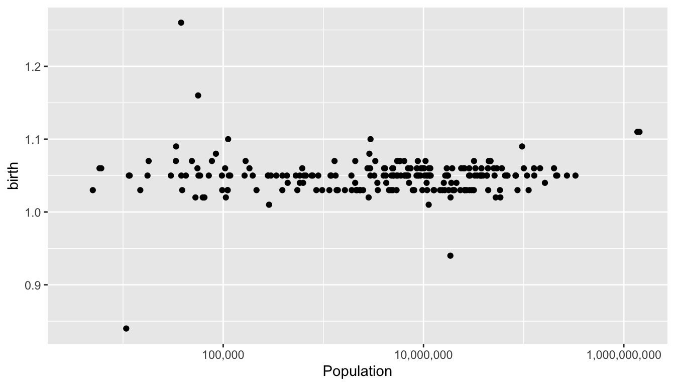
23.4 Sex Ratio Models
We may model the assigned sex data from a large collection of single human births as a similar to a collection of individual coin tosses with two outcomes, boy and girl. However, there are a number of modeling questions we might ask, including:
- Are the births independent (or conditionally independent)?
- Are boys and girls equally likely?
- If not equally likely, does each single birth have the same probability of being a boy, regardless of the family, the birth order, and the sexes of previous children in the family?
- Do different families have different probabilities that each child is a boy?
- Within a family, are the probabilities of having a boy the same, or do they change over time?
- Does the sex of the previous child affect the probability of the sex of the next child?
We will explore a few models using part of Geissler’s Saxony data looking at families with sex assigned at birth for eight children.
23.4.1 Data Summary
Here is a table that shows the counts.
g8 = read_csv("data/geissler.csv") %>%
  filter(size == 8)

library(kableExtra)
kable(g8) %>%
  kable_styling(position = "left", full_width = FALSE,
bootstrap_options = c("condensed","striped"))| boys | girls | size | freq |
|---|---|---|---|
| 0 | 8 | 8 | 161 |
| 1 | 7 | 8 | 1152 |
| 2 | 6 | 8 | 3951 |
| 3 | 5 | 8 | 7603 |
| 4 | 4 | 8 | 10263 |
| 5 | 3 | 8 | 8498 |
| 6 | 2 | 8 | 4948 |
| 7 | 1 | 8 | 1655 |
| 8 | 0 | 8 | 264 |
Before exploring models, examine the data graphically and numerically.
ggplot(g8, aes(x = boys, y = freq)) +
  geom_col(width = 1, color = "black", fill = "royalblue") +
  scale_x_continuous(breaks = 0:8) +
  xlab("# of boys") +
  ggtitle("# of Boys in Geissler Data Families of 8")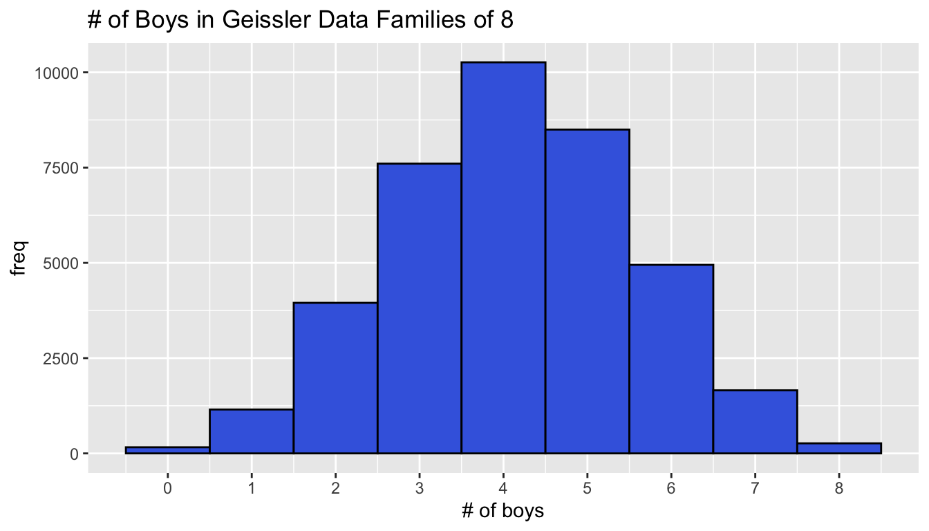
Calculate the total number of boys and girls by finding the number in each family and summing. Other data summaries are based on these values.
g8_sum = g8 %>%
  summarize(boys = sum(boys*freq),
            girls = sum(girls*freq),
            children = boys + girls,
            families = sum(freq),
            sex_ratio = 100 * boys/girls,
            p_boy = boys/children,
            p_girl = girls/children)

print(g8_sum, n = Inf)
# A tibble: 1 × 7
boys girls children families sex_ratio p_boy p_girl
<dbl> <dbl> <dbl> <dbl> <dbl> <dbl> <dbl>
1 158790 149170 307960 38495 106. 0.516 0.484g8_sum %>%
mutate(sex_ratio = round(sex_ratio,1),
p_boy = round(p_boy,3),
p_girl = round(p_girl,3)) %>%
kable() %>%
kable_styling(position = "left", full_width = FALSE,
bootstrap_options = c("condensed","striped"))| boys | girls | children | families | sex_ratio | p_boy | p_girl |
|---|---|---|---|---|---|---|
| 158790 | 149170 | 307960 | 38495 | 106.4 | 0.516 | 0.484 |
23.5 Simple Binomial Model
The simplest binomial model assumes that all births are independent, and that the probability of a boy for each birth is some value \(p\). Furthermore, the model treats this data as if the number of total children is fixed at eight. There are 38,495 families. If \(X_i\) is the number of boys in the \(i\)th family, the model is
\[ X_i \sim \text{i.i.d}\ \text{Binomial}(8,p) \]
The abbreviation i.i.d represents independent and identically distributed.
There are a number of assumptions associated with this model.
- All births are independent.
- All births have the same probability of being assigned as a boy.
- The family sizes are fixed at eight.
Note that this final assumption depends on behavior of people. Namely, it assumes that families do not base the decision as to whether to have additional children on the sexes of the previous children. This assumption is questionable (but not checkable from the data). These assumptions also do not allow there to be heterogeneity among families (some families with greater tendencies to produce boys and others for girls).
Under this model, there is only one parameter to estimate, namely \(p\). The natural estimate is the sample proportion: \[ \hat{p} = \frac{ \text{# of boys}}{\text{# of children}} \] Using the data, this is \(\hat{p} = 158,790 / 307,960 \doteq 0.516\).
This also is the maximum likelihood estimate.
Let’s examine how to calculate the maximum likelihood.
The likelihood for each family with x boys is \(L(p \,\mid\,x)\)
which we calculate with dbinom(x,8,p)
for each x from \(0,\ldots,8\).
These likelihoods are multiplied together for all families.
If the likelihood from the \(i\)th family is \(L(p \,\mid\,x_i)\),
the overall likelihood is
\[
\prod_{i=1}^n L(p \,\mid\,x_i)
\]
Each factor will be identical for families with the same number of boys.
If the number of families with \(x\) boys is \(n_x\)
where \(\sum_x n_x = n\),
the likelihood can also be written as
\[
L(p) = \prod_{x=0}^8 L(p \,\mid\,x)^{n_x}
\]
The likelihood is a product of thousands of numbers less than 1 and will be very small.
The log-likelihood, \(\ell(p \,\mid\,x) = \ln L(p \,\mid\,x)\),
will be much more stable to calculate numerically.
\[
\ell(p) = \sum_{x=0}^8 n_x\, \ell(p \,\mid\,x)
\]
The value of \(p\) that maximizes \(\ell(p)\) will also maximize \(L(p)\).
Here is a graph of the log-likelihood which is maximized at \(\hat{p} = 0.516\).
n = g8 %>% pull(freq)
x = g8 %>% pull(boys)
p = seq(0.5,0.53,0.001)
logl = numeric(length(p))
for ( i in seq_along(p) )
  logl[i] = sum( n * dbinom(x, 8, p[i], log = TRUE) )

tibble(p,logl) %>%
ggplot(aes(x=p, y=logl)) +
  geom_line() +
  geom_vline(xintercept = pull(g8_sum,p_boy),
             color = "red",
             linetype = "dashed") +
  geom_hline(yintercept = sum( n * dbinom(x, 8, pull(g8_sum,p_boy), log = TRUE) ),
             color = "red", linetype = "dotted") +
  ylab("log-likelihood")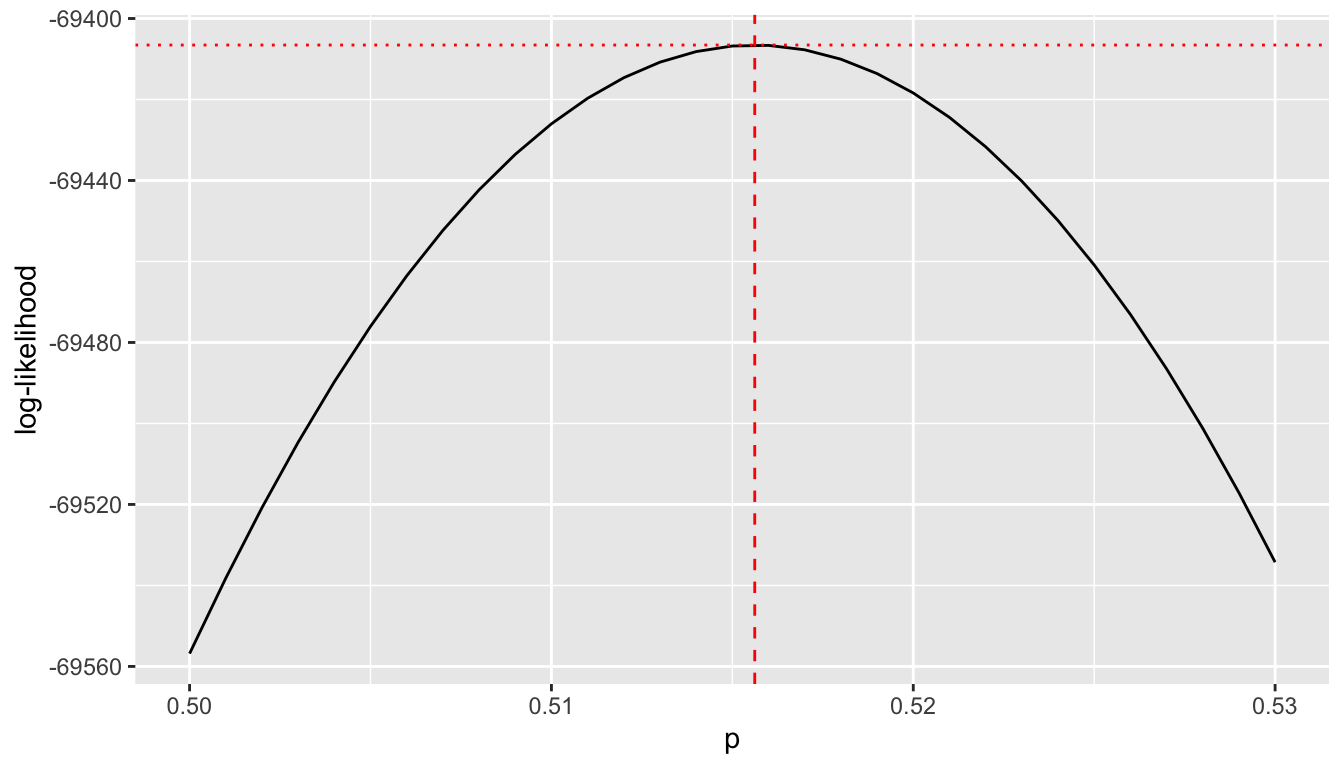
23.5.1 Numerical Optimization
We found the maximum likelihood estimate by using a formula.
Another approach is numerical optimization.
The function optim() is a general purpose optimization function.
Here is an example on how to use it for this problem.
We create a function which calculates the log-likelihood as a function of \(p\).
## log-likelihood
## 0 < p < 1 is a single value
## n is the data vector which has the number of outcomes from 0 to size
f = function(p, n)
{
  size = length(n) - 1
  x = 0:size
  return ( sum( n * dbinom(x, size, p, log = TRUE) ) )
}

## optim finds the minimum by default
## control = list(fnscale = -1) means the function minimizes -1 * f
##   which maximizes f

p0 = 0.5 ## initial guess
opt = optim(p0, f, n=n, control = list(fnscale = -1) )
Warning in optim(p0, f, n = n, control = list(fnscale = -1)): one-dimensional optimization by Nelder-Mead is unreliable:
use "Brent" or optimize() directly## par is the estimate
## value is the log-likelihood
## convergence = 0 means the optimization converged (it worked)
opt$par
[1] 0.515625
$value
[1] -69406.55
$counts
function gradient
24 NA
$convergence
[1] 0
$message
NULL## check
## the numerical result has a stopping rule
## and may stop before the theoretical optimum is reached
round(opt$par, 6)[1] 0.515625[1] 0.51561923.5.2 Goodness of Fit
Does the simple binomial model fit the data? We can compare the actual relative frequencies with the binomial probabilities. Here are the calculations and a graph.
p_boy = pull(g8_sum,p_boy)

g8 = g8 %>%
  mutate(emp_p = freq/sum(freq),
         binom_p = dbinom(boys, 8, p_boy),
         difference = emp_p - binom_p)

print(g8, n=Inf)
# A tibble: 9 × 7
boys girls size freq emp_p binom_p difference
<dbl> <dbl> <dbl> <dbl> <dbl> <dbl> <dbl>
1 0 8 8 161 0.00418 0.00303 0.00115
2 1 7 8 1152 0.0299 0.0258 0.00412
3 2 6 8 3951 0.103 0.0961 0.00649
4 3 5 8 7603 0.198 0.205 -0.00719
5 4 4 8 10263 0.267 0.272 -0.00577
6 5 3 8 8498 0.221 0.232 -0.0112
7 6 2 8 4948 0.129 0.123 0.00508
8 7 1 8 1655 0.0430 0.0375 0.00545
9 8 0 8 264 0.00686 0.00500 0.00186gbinom(8,p_boy) +
geom_segment(aes(x = boys + 0.1, y = emp_p,
xend = boys + 0.1, yend = 0),
data = g8, color = "red") +
scale_x_continuous(breaks = 0:8) +
ggtitle("Comparison Between Empirical and Binomial",
subtitle = "empirical = red, binomial = blue") +
xlab("# of boys")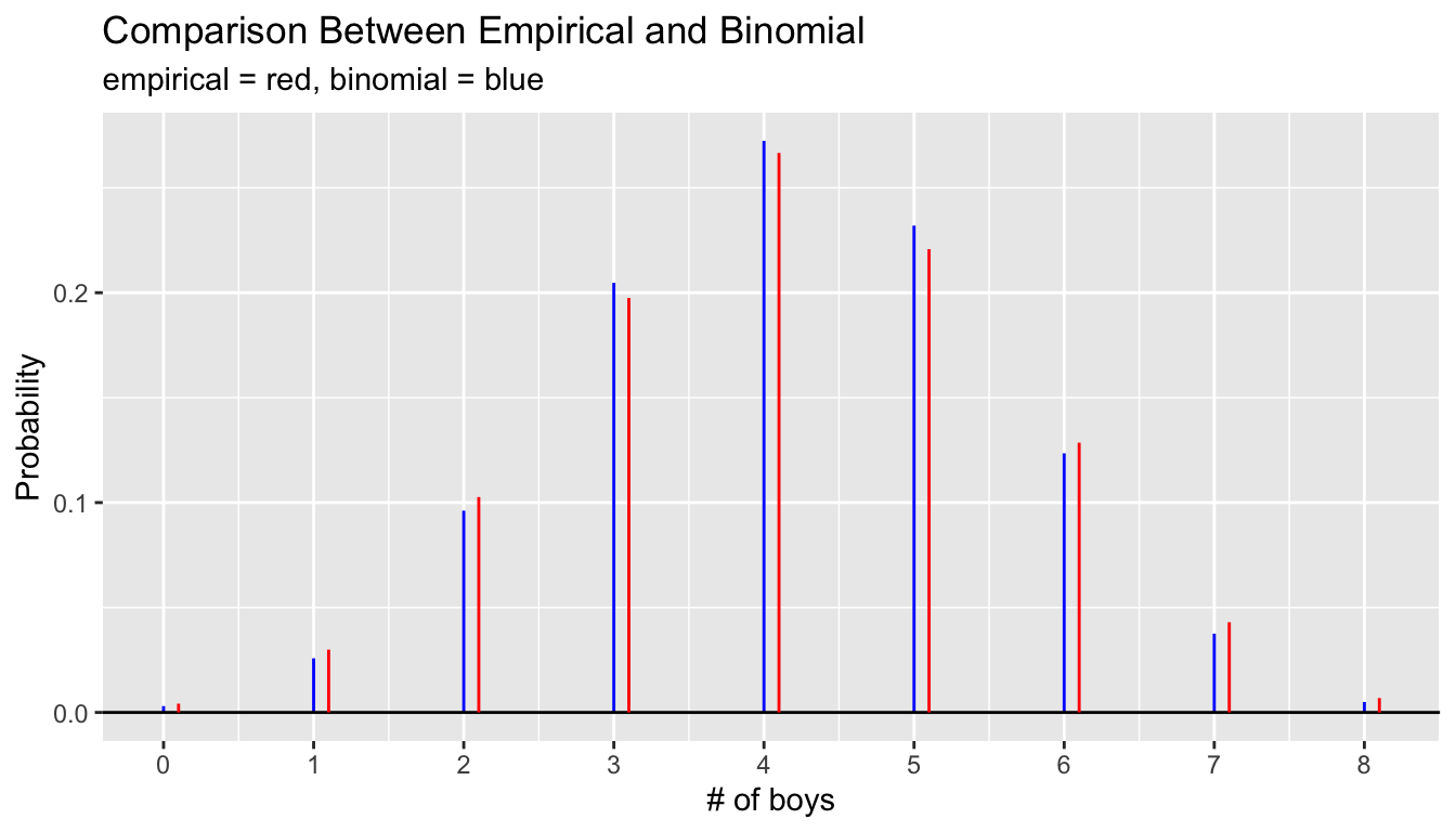
Notice that the observed proportions are slightly larger than the binomial predictions in the tails and slightly smaller in the middle of the distribution. The differences are not large, the largest being about 0.011 between the observed proportion of 0.221 and binomial model probability of 0.232 for the outcome of 5 boys and 3 girls. However, with the large sample size of 38,495, if the true probability was 0.232 that a family with 8 children in this population would have 5 boys and 3 girls, then the standard error of the observed proportion is only about 0.0021. This observed difference is nearly five times as large as the standard error. The normal distribution is an excellent approximation to the sample proportion for such a large sample size, which indicates very strong evidence against the simple binomial model. Something else is going on.
The distribution of observed numbers of boys per family is, just slightly, more variable than what the binomial model predicts.
g8 %>%
  summarize(p_boy = sum(boys*freq)/sum(8*freq),
            mu = 8*p_boy,
            sd_empirical = sqrt( sum( (boys - mu)^2 * emp_p ) ),
            sd_binomial = sqrt(8*p_boy*(1-p_boy)))
# A tibble: 1 × 4
p_boy mu sd_empirical sd_binomial
<dbl> <dbl> <dbl> <dbl>
1 0.516 4.12 1.47 1.41Statisticians use the term overdispersion to describe this situation. The next model is one possible way to explain the apparent overdispersion in the observed data.
23.6 Beta Binomial Model
One of the key assumptions of the previous model is that each single birth within a family had the same probability of being assigned as a boy. But what if this probability varied among the families? A model which assumes heterogeneity among the single birth boy probability values for each family may be described in the following way:
- Family \(i\) draws a random \(p_i\) from a continuous probability distribution;
- Given the value of \(p_i\), the number of boys in a family of eight has a binomial distribution.
\[ p_i \,\mid\,\alpha, \beta \sim \text{Beta}(\alpha,\beta) \] \[ X_i \,\mid\,p_i \sim \text{Binomial}(n,p_i) \]
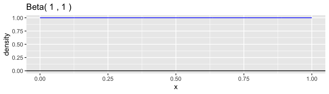
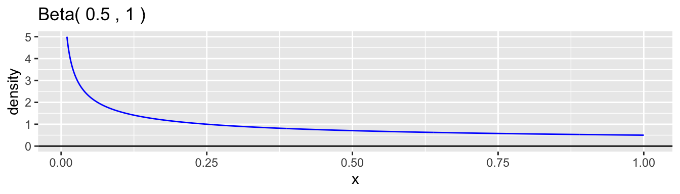
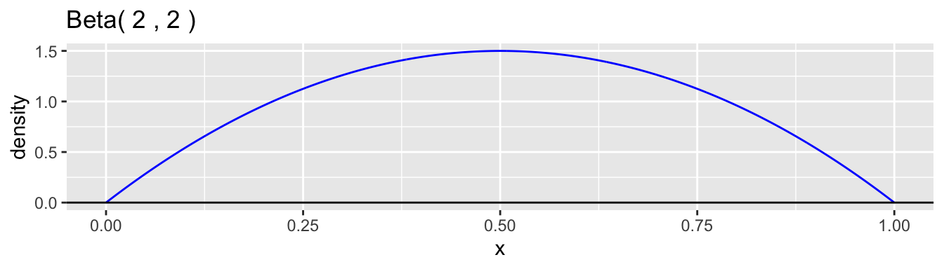
The beta distribution family is a common choice for the continuous probability distribution for \(p\). This distribution has support on the interval \((0,1)\) and allows a variety of shapes. Each beta distribution is described by two positive parameters, \(\alpha\) and \(\beta\), which are difficult to interpret individually, but are clearly defined in the formula for the probability density. \[ f(p) = \frac{p^{\alpha-1}(1-p)^{\beta-1}}{B(\alpha,\beta)}, \quad 0 < p < 1 \] The expression \(B(\alpha,\beta)\) is simply a normalizing constant so that the density has a total area of one. Here are graphs of a few examples of beta densities.
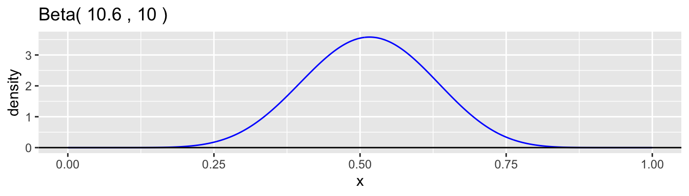
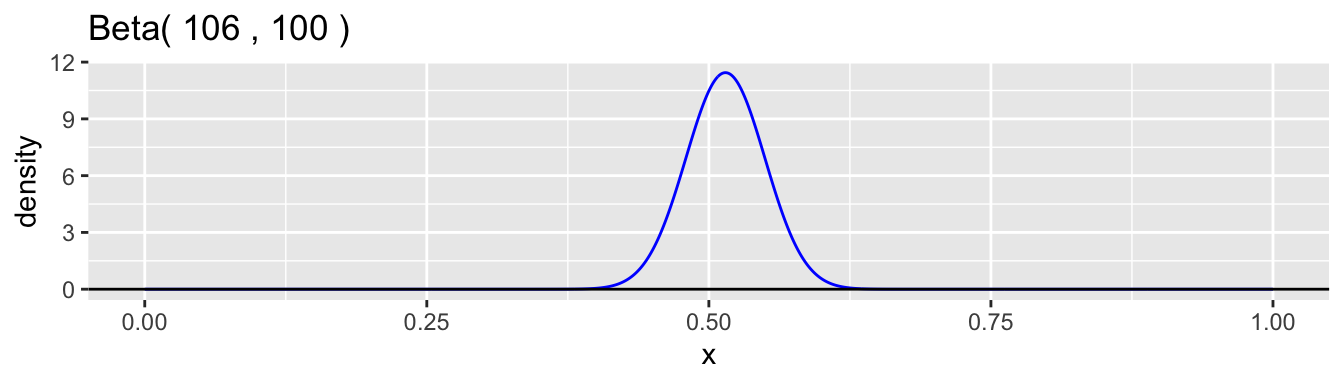
The mean and variance of a beta distribution are: \[ \mu = \frac{\alpha}{\alpha + \beta} \qquad \text{and} \qquad \sigma^2 = \frac{\alpha\beta}{(\alpha+\beta)^2(\alpha+\beta+1)} \] A common reparametrization is to use \(\mu\) and \(\phi = \alpha + \beta\), so that \(\alpha = \phi\mu\) and \(\beta = \phi(1-\mu)\). With this reparameterization, the variance is \(\sigma^2 = \mu(1-\mu)/(\phi+1)\). Examining the moments helps to understand better how to interpret the values of \(\alpha\) and \(\beta\). The ratio \(\alpha/\beta\) equals \(\mu/(1-\mu)\) and so is related, in our case study, to the relative proportions of boys to girls at birth, which is the sex ratio. We would expect this ratio to be close to 1.06 in our data example. The parameter \(\phi = \alpha + \beta + 1\) is inversely proportional to the variance while holding the mean constant. A low value of \(\phi\) corresponds to a high degree of heterogeneity in the probability of a boy among families. The higher the value is, the less heterogeneity there is and the closer the model approaches the simple binomial model.
While it is useful to think about the Beta-Binomial model as a two step process, we can also write the probability mass function out for \(X\) directly.
\[ X_i \,\mid\,\alpha,\beta \sim \text{Beta-Binomial}(n,\alpha,\beta), \quad \text{for all $i$} \] \[ \mathsf{P}(X_i = x) = \binom{n}{x} \frac{B(x+\alpha,n-x+\beta)}{B(\alpha,\beta)}, \quad \text{for $x=0,1,\ldots,n$} \] where \(\alpha>0\) and \(\beta>0\).
There is an integral expression for the beta function, \(B\).
\[
B(\alpha,\beta) = \int_0^1 p^{\alpha-1}(1-p)^{\beta-1}\, \mathrm{d}p
\]
More useful to us is the R function lbeta() which calculates the natural log of this beta function.
A second useful R function for this distribution is lchoose()
which calculate the natural log of the binomial coefficient.
With these functions,
we can write a function analogous to dbinom()
to compute the probability mass function of the beta-binomial distribution.
## beta-binomial density
dbb = function(x,n,a,b,log=FALSE)
{
  log_d = lchoose(n, x) +
    lbeta(x+a, n-x+b) -
    lbeta(a, b)
  if ( log )
    return ( log_d )
  return ( exp( log_d ) )
}
23.6.1 Parameter Estimation
Unlike the binomial model where there is a simple formula from the data for the maximum likelihood estimate of the parameter \(p\), no such formulas exist for \(\alpha\) and \(\beta\). However, we can use numerical optimization to determine these values. The block below defines functions for this calculation.
mbb()is a helper function which returns the sample mean and variances from a vector of counts of the number of observed random variables with each outcome from 0 to \(n\), such as thefreqcolumn of the data from our example.lmpbb()calculates the log-likelihood of the data using the \((\mu,\phi)\) parameterization.mlebb()finds the maximum likelihood estimates of the parameters in the beta-binomial model.
## This function assumes that the sample x_1,\ldots,x_m
## (all assumed from the same beta-binomial distribution)
## has been summarized into a vector of length n+1
## with the tabulated counts for each outcome from 0 to n
## The function returns the MLEs of the mean and variance
mbb = function(x)
{
  n = length(x) - 1
  m = sum(x)
  mx = sum((0:n)*x)/m
  vx = sum(x*(0:n - mx)^2)/m
  return(tibble(mx,vx))
}

## Log-likelihood function for (mu,phi)
## x are the counts from 0 to n
## theta = c(mu,phi)
lmpbb = function(theta,x)
{
  mu = theta[1]
  phi = theta[2]
  alpha = mu*phi
  beta = (1-mu)*phi
  n = length(x) - 1
  return( sum(x*dbb(0:n,n,alpha,beta,log=TRUE)) )
}

## Use optim to find mle estimates of alpha and beta from counts
## Use method of moments to start.
## Find mu and phi. Then translate to alpha and beta.
## If the returned convergence is not 0,
##   then there was an error in the optimization
mlebb = function(x)
{
  n = length(x)-1
  moments = mbb(x)
  mx = moments$mx
  vx = moments$vx
  mu_0 = mx/n
  phi_0 = (n*n*mu_0*(1-mu_0) - vx)/(vx - n*mu_0*(1-mu_0))
  tol = 1e-7
  opt = optim(c(mu_0,phi_0),lmpbb,x=x,
              control = list(fnscale=-1),
              method = "L-BFGS-B",
              lower = c(tol,tol),
              upper = c(1-tol,Inf))
  df = tibble(
    mu = opt$par[1],
    phi = opt$par[2],
    alpha = mu*phi,
    beta = (1-mu)*phi,
    logl = opt$value,
    convergence = opt$convergence)

  return( df )
}
Let’s examine the fit of this model to our data.
# A tibble: 1 × 6
     mu   phi alpha  beta    logl convergence
  <dbl> <dbl> <dbl> <dbl>   <dbl>       <int>
1 0.516 85.2 43.9 41.3 -69337. 0[1] 1.064492Note that the estimate for \(\mu\) matches the binomial estimate for \(\hat{p}\). The ratio of the estimated parameters \(\alpha/\beta\) matches the observed sex ratio, 1.06. A plot of the beta density for the estimated \(\alpha\) and \(\beta\) helps to better understand what the model says about heterogeneity.
gbeta(bb_8$alpha, bb_8$beta, a = 0.3, b = 0.7) +
  geom_beta_fill(bb_8$alpha, bb_8$beta, a = 0.3, b = 0.7, fill = "blue") +
  ggtitle("Beta Density Estimate")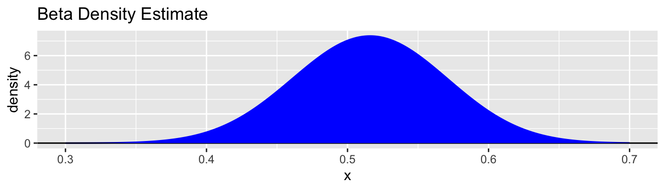
[1] 0.410 0.479 0.552 0.620In the context of the beta-binomial model and this data:
- The overall probability of a boy in a single birth is estimated at 0.516.
- There is variability from family to family in this distribution.
- Half the families have the boy probability vary between about 0.479 and 0.552.
- Most (95%) of the families have the boy probability vary between 0.41 and 0.62.
23.6.2 Goodness of Fit
How do the beta-binomial probability estimates compare to the observed proportions?
## Calculate the beta-binomial estimates
g8 = g8 %>%
  mutate(bb_p = dbb(boys, 8, bb_8$alpha, bb_8$beta),
         bb_diff = emp_p - bb_p)

g8 %>%
  print(n=Inf)
# A tibble: 9 × 9
boys girls size freq emp_p binom_p difference bb_p bb_diff
<dbl> <dbl> <dbl> <dbl> <dbl> <dbl> <dbl> <dbl> <dbl>
1 0 8 8 161 0.00418 0.00303 0.00115 0.00418 0.00000398
2 1 7 8 1152 0.0299 0.0258 0.00412 0.0304 -0.000498
3 2 6 8 3951 0.103 0.0961 0.00649 0.101 0.00142
4 3 5 8 7603 0.198 0.205 -0.00719 0.201 -0.00346
5 4 4 8 10263 0.267 0.272 -0.00577 0.260 0.00618
6 5 3 8 8498 0.221 0.232 -0.0112 0.226 -0.00481
7 6 2 8 4948 0.129 0.123 0.00508 0.128 0.000996
8 7 1 8 1655 0.0430 0.0375 0.00545 0.0430 -0.0000511
9 8 0 8 264 0.00686 0.00500 0.00186 0.00664 0.000218 ggplot(g8) +
geom_segment(aes(x = boys + 0.1, y = emp_p,
xend = boys + 0.1, yend = 0),
color = "red") +
geom_segment(aes(x = boys, y = bb_p,
xend = boys, yend = 0),
data = g8, color = "blue") +
scale_x_continuous(breaks = 0:8) +
ggtitle("Comparison Between Empirical and Beta-Binomial",
subtitle = "empirical = red, beta-binomial = blue") +
xlab("# of boys") +
ylab("probability")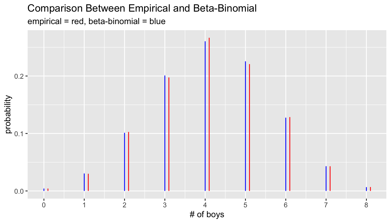
# A tibble: 1 × 9
   boys girls  size  freq emp_p binom_p difference  bb_p bb_diff
  <dbl> <dbl> <dbl> <dbl> <dbl>   <dbl>      <dbl> <dbl>   <dbl>
1     4     4     8 10263 0.267   0.272   -0.00577 0.260 0.00618
The largest difference between observed proportions and the model predictions occurs at the middle with four boys and four girls where the observed frequency of 0.267 is 0.007 larger than the predicted frequency of 0.260. This is a small difference, but it is about three times as large as the standard error as the very large sample size allows for high precision.
There are a number of ways that the model might be adjusted. First, allow a different density model for \(p\) than the beta. When \(\mu\) is nearly 0.5 as in this setting, the beta density is very nearly symmetric. If the true distribution were skewed, this could lead to model misfit. Second, notice, interestingly, that the empirical distribution is larger than the model prediction for even numbers of boys and girls and less when there are odd numbers of each. Perhaps this might be explained by the choices a family makes on whether or not to continue having children, which we ignore. A third possibility is allowing \(p\) to vary within families. The Geissler data set, however, does not allow us to explore this.
23.6.3 Likelihood Ratio Test
We have seen that the beta-binomial model fits the observed proportions more closely than the binomial model, but as the model has a larger number of parameters, we expect this. Is the difference statistically discernible?
Recall that the log-likelihood using the simple binomial model was \(-69,406.55\). With the beta-binomial model, the log-likelihood is \(-69,337.23\). The LRT test statistic is twice the difference, or about 138.65. There is only one parameter difference between the models and the binomial model may be considered as a special case of the beta-binomial model where \(\mu = p\) and \(\phi \rightarrow +\infty\) (so the variance approaches zero). The p-value is the area to the right of 138.65 under a chi-square distribution with one degree of freedom, which is essentially zero. Recall a chi-square distribution with one degree of freedom is the distribution of the square of a standard normal random variable, so this test statistic corresponds to a standard normal random variable being more than 11.7 (the square root of the test statistic) standard deviations from the mean, which has no measureable probability.
23.7 Further Analysis
Lecture and future homework assignments with explore further the other data sets and alternative models.
23.8 Questions
- Examine the Geissler data for different family sizes.
- How do the estimates of \(p_{\text{boy}}\) and the sex ratio differ?
- Is the beta-binomial model as much a better fit than the simple binomial model in each instance?
- Examine the French sex ratio data from the late 1940s.
- What are the overall proportions of boys and girls?
- What is the estimated secondary sex ratio?
- Determine the number of boys and girls born in each birth order.
- Determine the number of families for each family size.
- What are the distributions of the numbers of boys and girls?
- Compare the binomial and beta-binomial models for a fixed family size.
- How do the results compare to the Geissler data set?
- For each family size, determine the proportion that have another child.
- How do these proportions vary based on the family composition?
- Compare the probability that the next child is a girl among families with the same size, but different compositions of boys and girls, given that there is another child.
Examine the Danish sex ratio data and answer the same questions.
Examine the world sex ratio data.
- What is the range of typical sex ratios.
- Which countries have unusually high or low sex ratios?
- Some countries have very small populations so that randomness can explain unusual sex rations. If you restrict attention to countries with a population greater then one million people, which countries are outliers? Can you offer possible explanations?
Malinvaud, Edmond (1955). Relations entre la composition des familles et le taux de masculinité. Journal de la société statistique de Paris, tome 96, p. 49-64↩︎