20 Normal Distributions

The normal distribution, recognized for its canonical bell-shaped density function, is the single most important continuous probability distribution for statistical inference and theory. The reason that the normal distribution has such importance is its role the central limit theorem, which states, roughly, that the distribution of sums of independent and identically distributed random variables can be well approximated by normal distributions under fairly general conditions when the sample sizes are sufficiently large. A precise statement of the central limit theorem describes a limiting behavior, but the practical importance is that for many distributions and reasonable sample sizes, the normal distribution approximation can be very accurate. There are extensions to the central limit theorem for cases where the independence and identical distribution conditions may be relaxed to various forms of weak dependence and some differences in distribution, but these considerations are not important for this discussion.

Many real continuous random variables have distributions that are well approximated by normal distributions. Some random variables whose distributions are not well fit by a normal distribution might be transformed, for example by taking logarithms, to obtain a better approximation. More importantly, even when variables themselves are not well approximated, many numerical summaries of moderately sized or larger random samples can be approximated well.

The remainder of this chapter introduces the normal distribution and R commands to work with it.

20.1 Parameters

Each normal distribution is described fully by two parameters: the mean (\(\mu\)) and standard deviation (\(\sigma\)), using conventional notation. The mean is the weighted average of the possible values of the random variable, weighted by the probability density of each value. The standard deviation is the square root of the variance. The density is centered at the mean and the mean is the balancing point. The standard deviation is a measure of scale.

If a random variable \(X\) has a normal distribution with mean \(\mu\) and standard deviation \(\sigma\), we often denote this \[ X \sim \text{Normal}(\mu, \sigma^2) \] where \(\sigma^2\) is the variance. Some texts will label the distribution with the standard deviation instead of the variance.

20.2 Normal Probability Density

The formula for the normal density is \[ f(x) = \frac{1}{\sigma\sqrt{2\pi}} \mathrm{e}^{- \frac{1}{2}\left( \frac{x - \mu}{\sigma} \right)^2 } \]

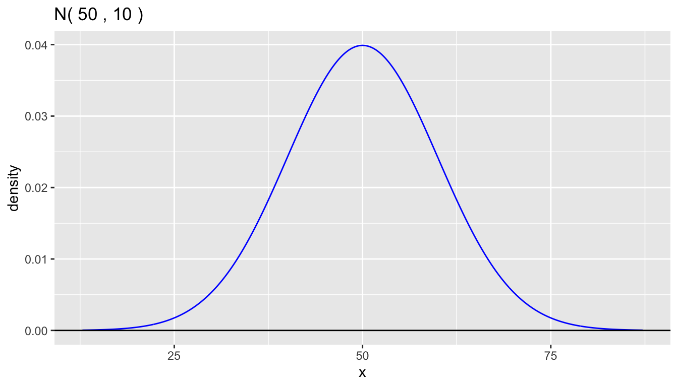
A graph of the density shows the bell-shaped curve.

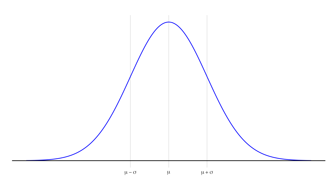
Every normal density has exactly the same shape.
The density curve is symmetric around the mean
- The median is equal to the mean
The locations one standard deviation below and above the mean are at the points of inflection where the slopes of tangent lines to the curve are steepest.
The total area under the density curve is equal to one, as it is for every probability density.
Probabilities are associated with areas under the density curve.

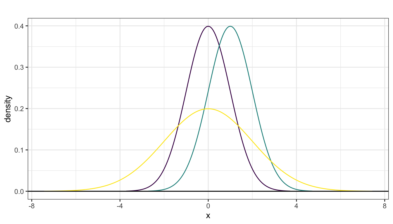
When multiple normal densities are drawn on the same axis, you can observe effects of modifying parameter values. The next plots displays densities from the following three normal distributions:

Purple: \(\text{Normal}(0,1)\)
Green: \(\text{Normal}(1,1)\) (shifted right of the purple density)
Yellow: \(\text{Normal}(0,2)\) (more spread out than the purple density)

20.3 Standard Normal Density

The standard normal density has mean \(\mu = 0\) and standard deviation \(\sigma = 1\).

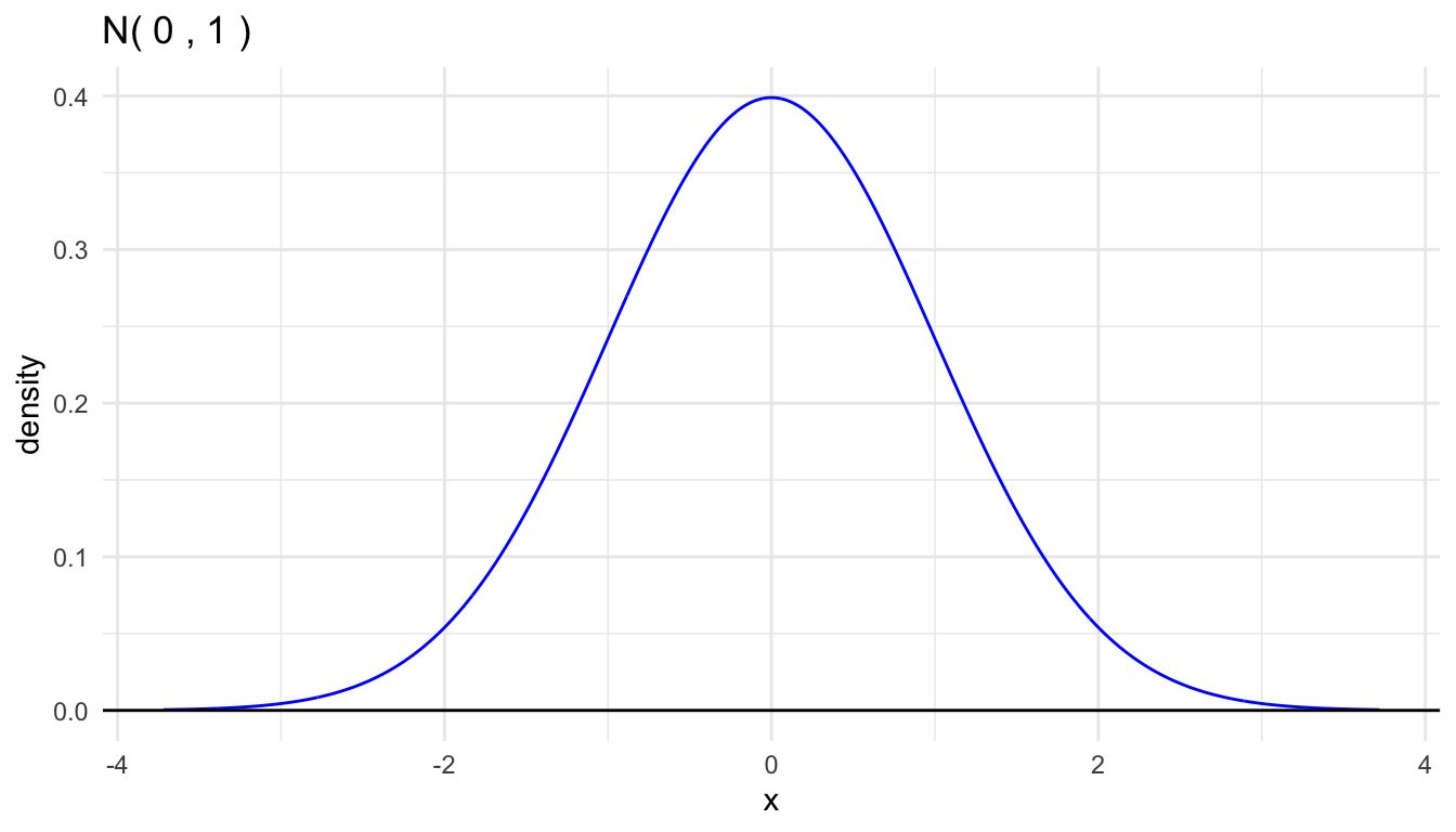
We conventionally use the symbol \(Z\) for a standard normal random variable. \[ Z \sim \text{Normal(0,1)} \]

Every normal random variable may be converted to a standard normal random variable by a linear transformation: substract the mean to center at zero and divide by the standard deviation to rescale. \[ Z = \frac{X - \mu}{\sigma} \]

Every normal random variable may be created by rescaling and recentering a standard normal random variable. \[ X = \mu + \sigma Z \]

20.4 Benchmark Normal Probabilities

Every normal random variable has the following benchmark areas:

The area within one standard deviation of the mean (between \(\mu - \sigma\) and \(\mu + \sigma\)) is approximately 68%.
The area within two standard deviations of the mean (between \(\mu - 2\sigma\) and \(\mu + 2\sigma\)) is approximately 95%.
The area within three standard deviations of the mean (between \(\mu - 3\sigma\) and \(\mu + 3\sigma\)) is approximately 99.7%.

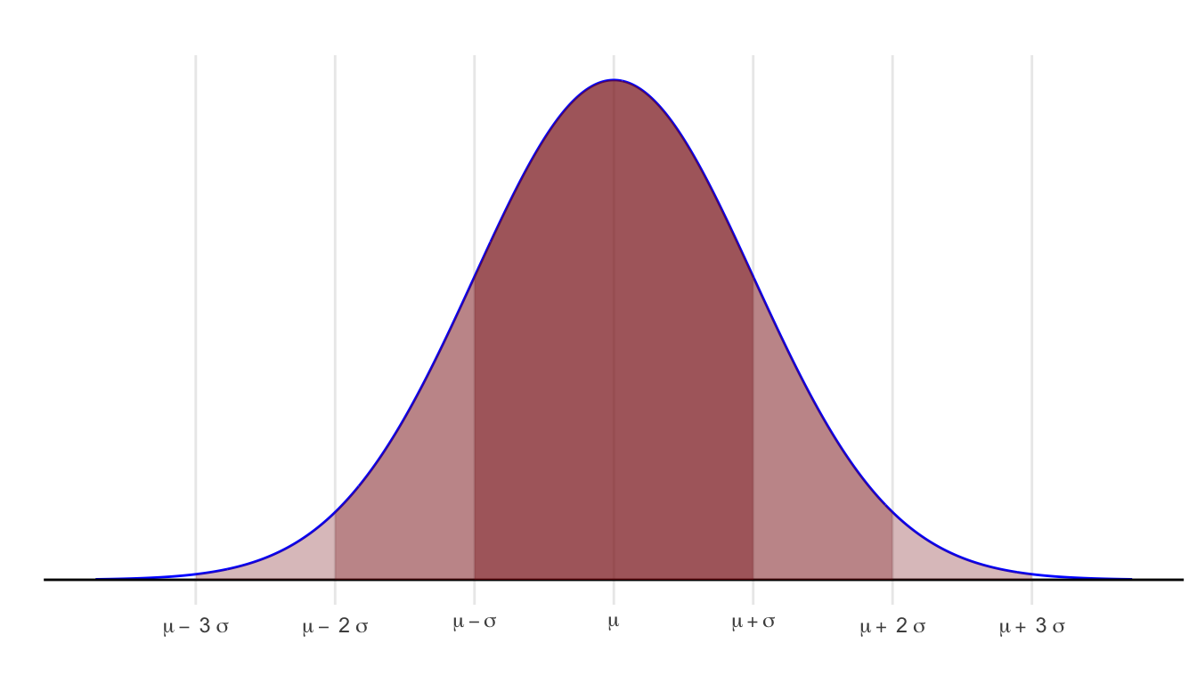
These benchmarks are easily extended to tail areas.

The area in the tail to the left (right) of \(\mu - \sigma\) (\(\mu + \sigma\)) is about 16%.
The area in the tail to the left (right) of \(\mu - 2\sigma\) (\(\mu + 2\sigma\)) is about 2.5%.

20.5 Normal CDF

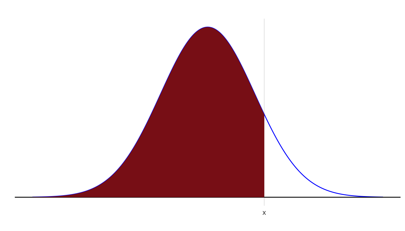
For any probability distribution, the cumulative distribution function (cdf) returns the probability that the random variable is less than or equal to the value. \[ F(x) = \mathsf{P}(X \le x) \]

Note:

For a continuous distribution like the normal, it does not matter if we use \(<\) or \(\le\) because the probability of being exactly at one value is zero (the area of a line segment is zero).
However, the distinction matters for discrete random variables. For a binomial random variable, \(\mathsf{P}(X < 3)\) and \(\mathsf{P}(X \le 3)\) differ by \(\mathsf{P}(X = 3)\).

For a normal distribution, this is the area to the left of \(x\) under the corresponding normal density.

For the standard normal curve, we use the special symbols \(\phi(z)\) for the density and \(\Phi(z)\) for the cdf:

\[ \phi(z) = \frac{1}{\sqrt{2\pi}} \mathrm{e}^{- \frac{z^2}{2}} \]

Using notation from calculus, \[ \Phi(z) = \int_{-\infty}^z \phi(t)\, \mathrm{d}t \]

Areas for any intervals are easily calculated in reference to the cdf.

left tail: \(\mathsf{P}(Z < z) = \Phi(z)\)
right tail: \(\mathsf{P}(Z > z) = 1 - \Phi(z)\)
finite interval: \(\mathsf{P}(a < Z < b) = \Phi(b) - \Phi(a)\)
outer area: \(\mathsf{P}(|Z| > a) = 2\Phi(-a)\) is \(a>0\) and \(1\) is \(a < 0\).

Areas for an arbitrary normal random variable are equivalent to a corresponding area under the standard normal curve, using the standardization change of variable.

If \(X \sim \text{Normal}(\mu, \sigma^2)\), then

\[ \mathsf{P}(X \le x) = \mathsf{P}\left(\frac{X - \mu}{\sigma} < \frac{x - \mu}{\sigma}\right) = \mathsf{P}\left(Z \le \frac{x - \mu}{\sigma}\right) \]

20.6 Central Limit Theorem

The random variables \(X_1, \ldots, X_n\) are independent and drawn from a distribution \(F\) where \(\mathsf{E}(X_i) = \mu\) and \(\mathsf{Var}(X_i) = \sigma^2\). The sample mean is a random variable defined as \[ \bar{X} = \frac{ \sum_{i=1^n} X_i }{ n } \] Then:

\(\mathsf{E}(\bar{X}) = \mu\)
\(\mathsf{Var}(\bar{X}) = \frac{\sigma^2}{n}\)
If \(n\) is large enough, then the distribution of \(\bar{X}\) is approximately normal.

20.6.1 Notes

The first two statements are true for any distribution \(F\) (where the mean and variance exist).
The accuracy of the approximation to the normal distribution depends both on the size of \(n\) and how close \(F\) itself is to normal.
- If \(F\) is normal, then the distribution of \(\bar{X}\) is also normal for any \(n\).
The strength of skewness in \(F\) is the single factor which most strongly affects the quality of the approximation.
- A distribution \(F\) with very strong skewness will typically require a larger \(n\) (maybe much larger \(n\)) for the approximation to be accurate.

20.7 Normal Calculations using R

There are several useful functions for working with the normal distribution in R. Each of these functions has the root norm and has as a prefix one of p, d, r, or q.

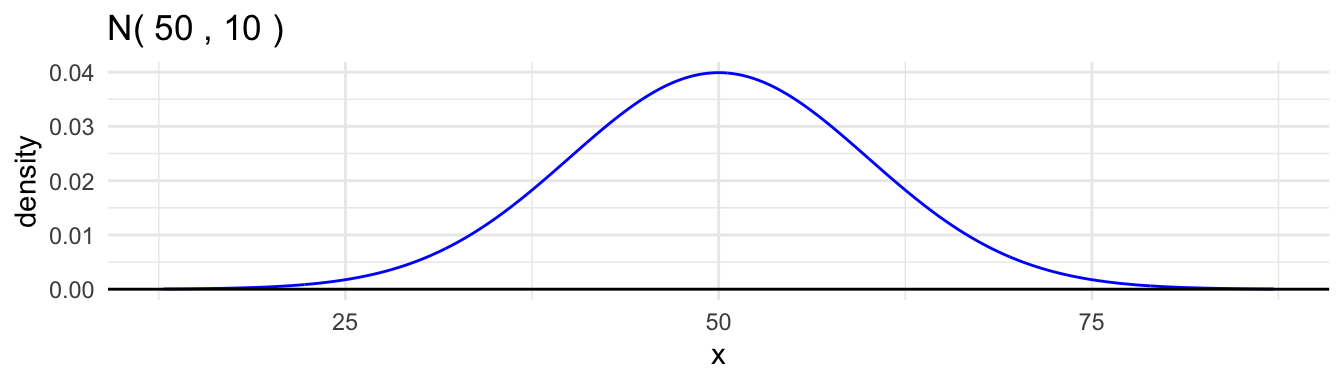
Here are examples for the \(\text{Normal}(50, 10^2)\) distribution.

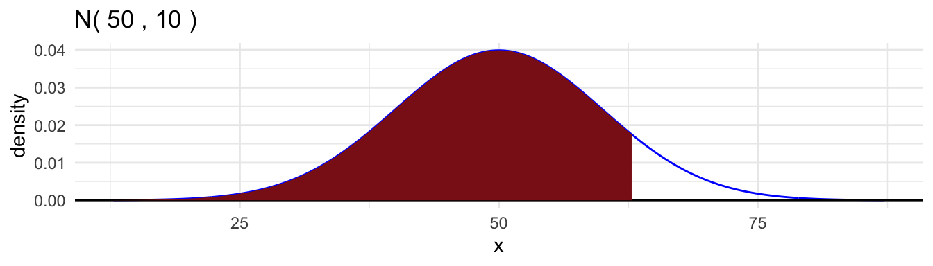
The cumulative distribution function, pnorm().

## directly
pnorm(40, 50, 10)

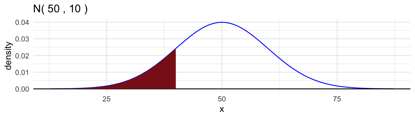
[1] 0.1586553

## using standardization
pnorm((40 - 50)/10)

[1] 0.1586553

The density function, dnorm()

dnorm(40, 50, 10)

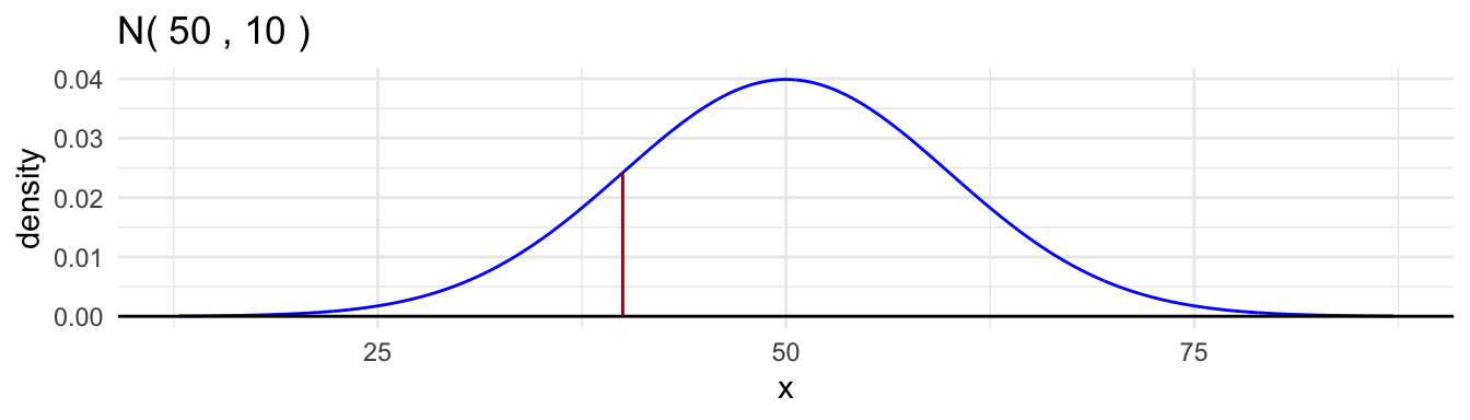
[1] 0.02419707

The quantile function, qnorm().

qnorm(0.9, 50, 10)

[1] 62.81552

Random samples, rnorm().

rnorm(15, 50,10)

 [1] 41.27094 42.13957 76.66895 46.20586 52.95887 43.18090 38.53184 41.31807
 [9] 39.57165 29.03125 52.20425 35.74484 57.34440 44.16928 48.15942

20.8 Graphing Normal Distributions

The file ggprob.R contains the definitions of several useful functions for graphing normal distributions.

gnorm() for creating a graph of a normal density
geom_norm_density() to add a normal density to a plot
geom_norm_fill() to shade in part of a normal density

Each function is compatible with ggplot2 functions.

Note: these functions are not part of a package and are not in base R. You need to source the code in ggprob.R just as you do with viridis.R.

Basic Usage

The first two arguments are \(\mu\) and \(\sigma\).

gnorm(50, 10)

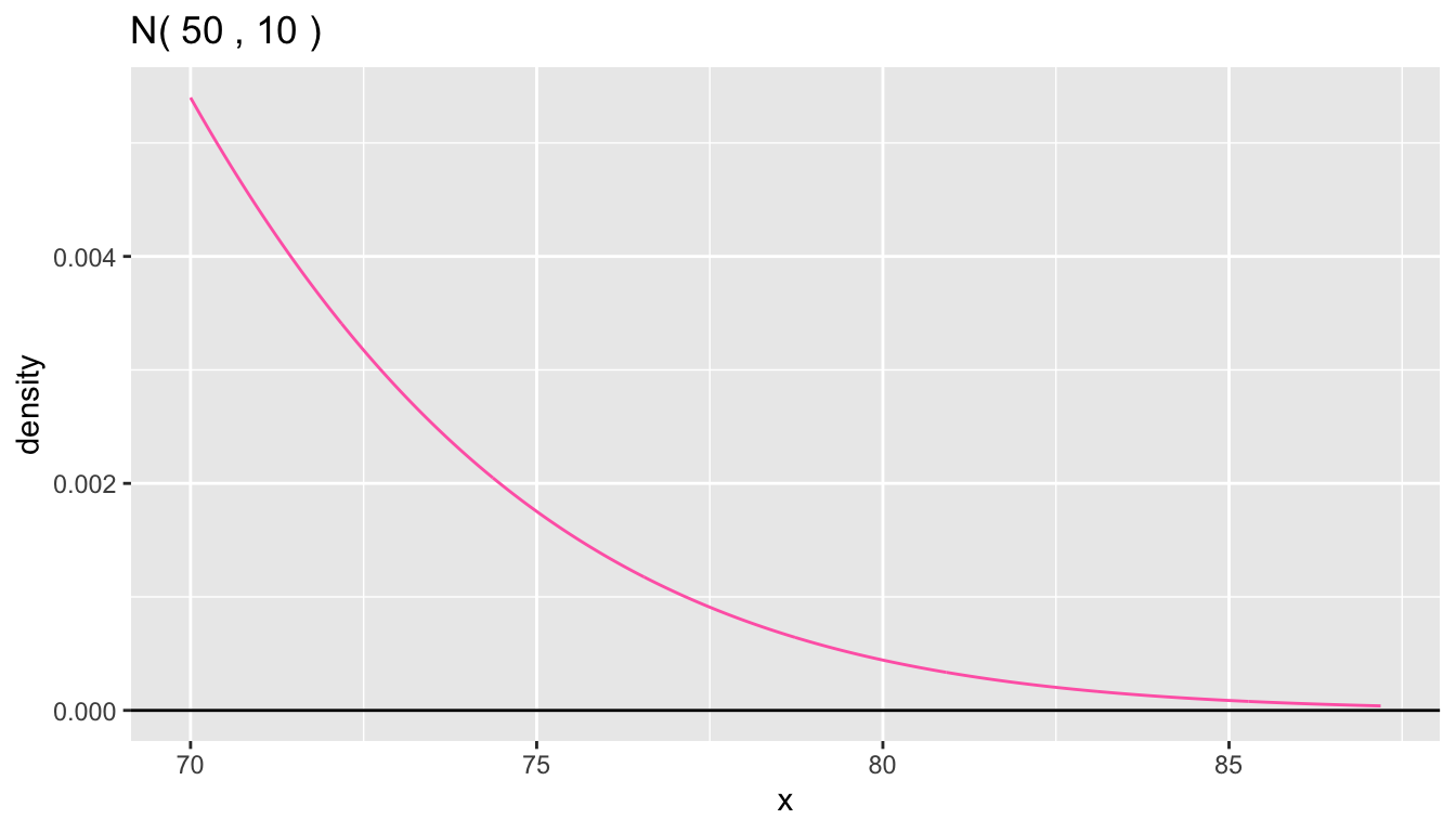
You can use the arguments a and b (or specify only one to use the default value of the other) to change the range for which the density is plotted. The argument color changes the color. Here is a plot of the upper right tail above 70 from the previous density plot.

gnorm(50, 10, a = 70, color = "hotpink")

You can add a layer with geom_norm_density() or other ggplot2 commands. Note that arguments to gnorm() are not aesthetics, so you need to repeat the mean and sd for each layer. Here is a plot with a variety of normal curves.

ggplot() +
  geom_norm_density(100,10, color = "blue") +
  geom_norm_density(120,10, color = "red") +
  geom_norm_density(110,20, color = "violet") +
  geom_hline(yintercept = 0) +
  ylab("density") +
  theme_bw()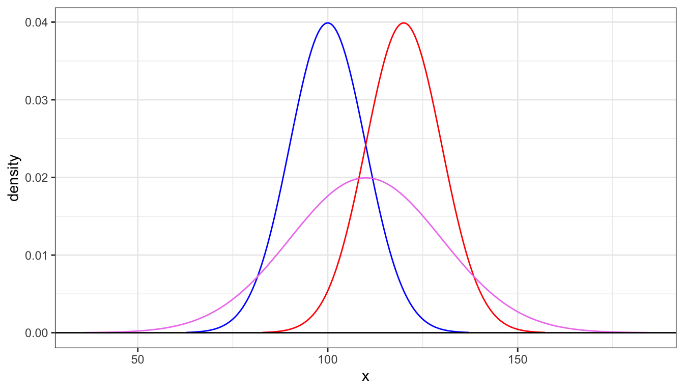

You can use geom_norm_fill() to draw a density where the area under the curve is filled. Specify fill and alpha to adjust these characteristics.

ggplot() +
  geom_norm_fill(100,10, fill = "cyan", alpha = 0.5) +
  geom_norm_fill(120,10, fill = "magenta", alpha = 0.5) +
  geom_hline(yintercept = 0) +
  ylab("density") +
  theme_bw()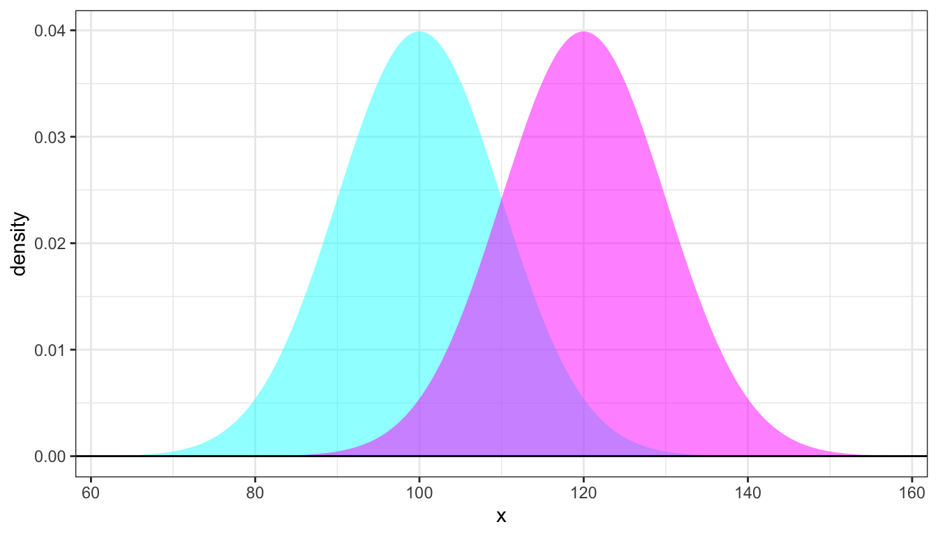

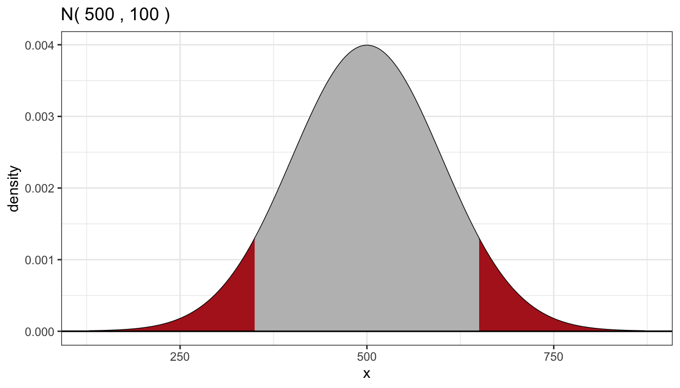
Use the arguments a and/ or b to shade in part of the density.

gnorm(500,100, color = "black") +
  geom_norm_fill(500,100, a = 650, fill = "firebrick") + ## right tail
  geom_norm_fill(500,100, b = 350, fill = "firebrick") + ## left tail
  geom_norm_fill(500,100, a = 350, b = 650, fill = "gray") + ## center
  geom_hline(yintercept = 0) +
  ylab("density") +
  theme_bw()