2 Prerequisites
2024-01-24
2.1 Online Textbooks
The online book R for Data Science (R4DS) is at https://r4ds.had.co.nz/ . The first author of the book, Hadley Wickham, is the primary author of the suite of R packages called the tidyverse that we will use extensively. There is also a paper version of the textbook. However, the online textbook has been edited more recently than the paper version and also uses a different numbering scheme for the chapters. This course will refer to the online version of R4DS exclusively.
A link to this online textbook is also available on the course website.
2.2 R and RStudio
You need the R statistical software package and the RStudio Desktop tool, an integrated development environment (IDE) for writing R code for the course. R is a programming language, developed by statisticians, that is very widely used for many data science applications. RStudio is software we will use which contains all of the tools needed to write and edit files, run R, make graphs, do data analysis, write reports, and render the reports into the HTML files you will need to upload for homework solutions, exams, and course projects. You will need to install both R and RStudio onto your computer. However, in this course we will never run R directly and will only interact with R through RStudio.
In 2022, the company RStudio changed its name to Posit, reflecting a more general scope of interest in data science that extends beyond the R language and includes other languages, such as Python. However, the RStudio IDE remains the name of the IDE we will use in the course.
2.2.1 Installing R
First install R, then install R Studio. The simplest way to do this is by following the instructions on the Posit web page.
Click on the link to the Posit download webpage: https://posit.co/downloads/
Click on a blue box which reads “Download R Studio”.
This takes you to a page with blue boxes to complete two steps:
- First, click on the blue box which reads “Download and install R”
- Follow all steps for your specific computer (details below)
- After R is installed, then click on the box which reads “Download R Studio Desktop for …” where the “…” should match your computer hardware and operating system.
- Follow steps to complete the installation
- First, click on the blue box which reads “Download and install R”
Note: In the installation process, you are strongly recommended to install the software in default locations on your computer. Do not install the software in the cloud, such as using OneDrive.
2.2.1.1 Default Installation Directories
I strongly recommend that you do not change the default directories for where to install R or RStudio. The software must be installed on your local computer and not in some cloud service for you to be able to run the software. Changing the default software location might lead to problems down the road if the software cannot find certain libraries, other packages, and so on. Successfully using R and RStudio from a location that is not the default one requires substantial expertise and care. Just use the default locations!
2.2.1.2 Detailed Installation Instructions for R
Clicking on the “Download and Install R” button should have taken you to the web page
which is a mirror of the main R web site. (Only use this link if the previous one fails.)
You should see a webpage where the top looks something like this:
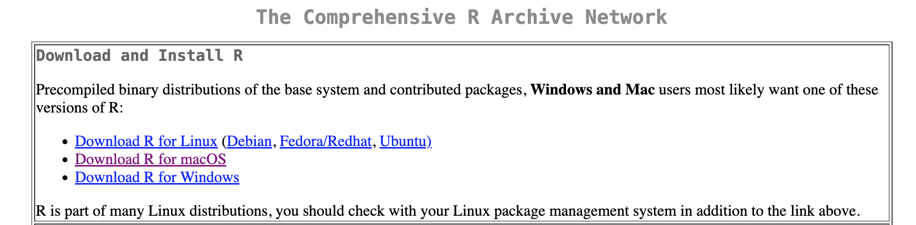
- Click on the link near the top of the page to the version of the software for your operating system.
- Install the latest version of R.
- If you have a Mac, it is important to select the correct version of the software.
- Recent Macs are built using the ARM64 architecture. If you such a Mac:
- download the most recent binary with a name like
R-X.X.X-arm64.pkg. (In January 2024, this isR-4.3.2-arm64.pkg.)
- download the most recent binary with a name like
- If your Mac has the older Intel-based CPUs, you want a different compiled version of the software.
- download the most recent binary with a name like
R-X.X.X-x86.pkg. (In January 2024, this isR-4.3.2-x86_64.pkg.)
- download the most recent binary with a name like
- In both cases:
- Double click the downloaded package and follow instructions.
- Use the default directories for installation.
- If you have Windows:
- Click on
base(orinstall R for the first time) - Click on the
Download R X.X.X for Windowslink (in January 2024, this is 4.3.2) - Double click the downloaded file and follow the instructions
- Click on
- If you have Linux:
- you probably know how to do what needs doing on your own
- ask me or a TA if you need help
Once you have R installed, do not open it directly. We will only interact with R through RStudio
2.2.2 Installing RStudio
The RStudio IDE is available from the Posit company website at https://posit.co/downloads/.
Click on the big blue
Download RStudiobutton in the upper right corner.The browser should be smart enough to detect your computer and will take you to a page with links for installation. If you already installed R as above, you can skip Step 1. Just click on the big blue button in Step 2, Install RStudio, that says **Download RStudio Desktop for ___** with your operating system filling in the blank. Click on the link to download and follow instructions. This will install the latest version of RStudio. As of January 2024, this is 2023.12.0+369.
2.2.3 Creating an R Studio Shortcut
As you will frequently use R Studio throughout the semester, it will be convenient to add a shortcut to R Studio on your computer.
On a Mac, drag the R Studio icon from your Applications folder to your Dock.
On a Windows computer, you can create a desktop short-cut by clicking the start button, finding the application, and then dragging it to your desktop.
2.2.4 Setting RStudio Defaults
While not strictly required, I strongly suggest that you change preferences in RStudio to never save the workspace so you always open with a clean environment (which makes your work reproducible).
See section 8.1 of R4DS at https://r4ds.had.co.nz/workflow-projects.html#what-is-real for some more background.
- Start RStudio
- Open RStudio preferences
- Open the Tools menu and then select Global Options
- (On a Mac, an alternative is to click on the RStudio menu and select Preferences…)
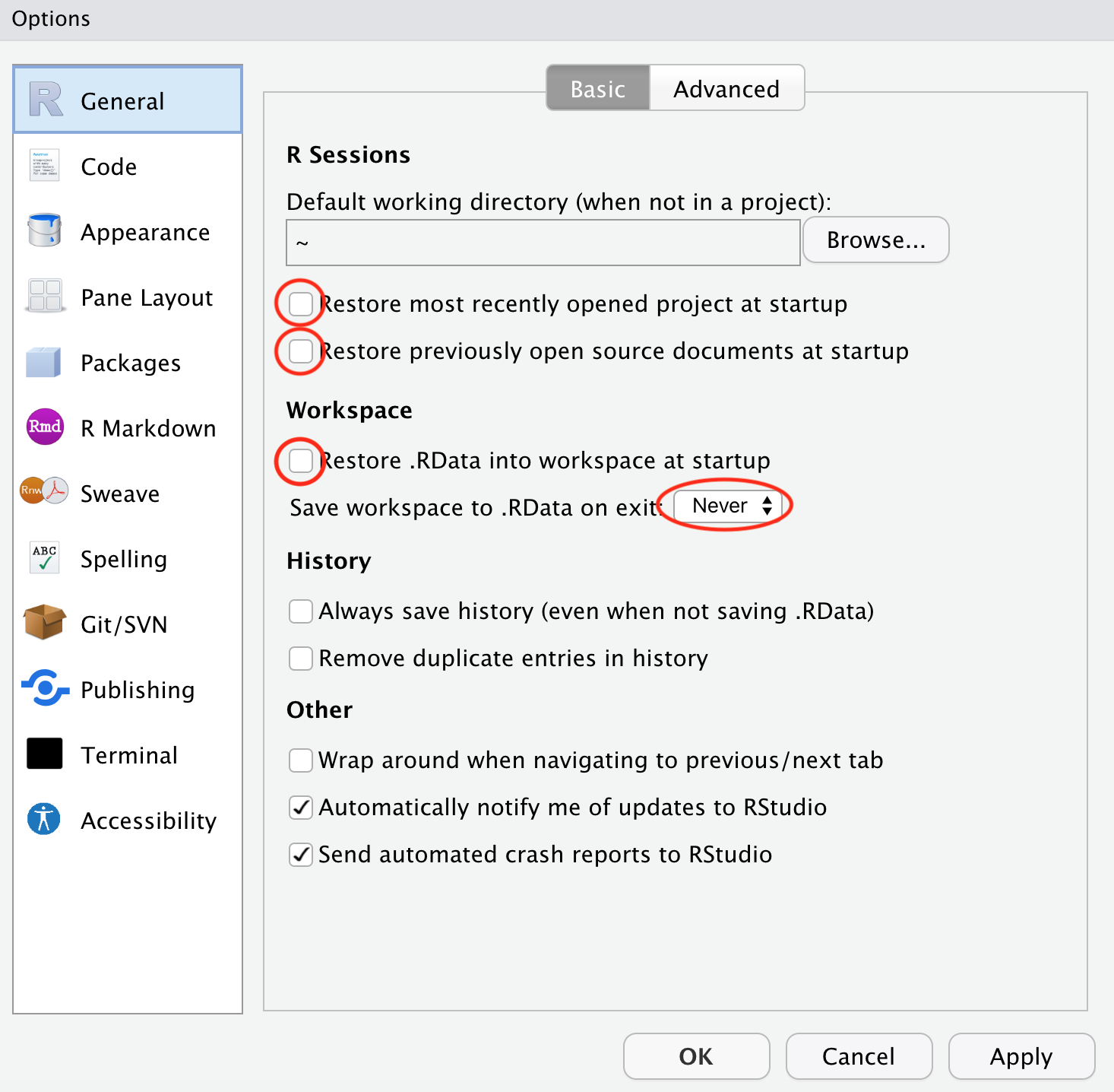
- Make sure the General button is highlighted from the left panel.
- Uncheck the three
Restoreboxes- Restore most recently opened project at startup
- Restore previously open source documents at startup
- Restore .RData into workspace at startup
- set
Save Workspace to .RData on exitto Never - Click OK at the bottom to save the changes and close the preferences window.
The reason for making these changes is that it is preferable for reproducibility to start each R session with a clean environment. You can restore a previous environment either by rerunning code or by manually loading a previously saved session.
The RStudio environment is modified when you execute code from files or from the console. If you always start fresh, you do not need to be concerned about things not working because of something you typed in the console, but did not save in a file.
You only need to set these preferences once.
There are many other preferences you can adjust as you learn more about RStudio and decide what to customize for yourself.
2.2.5 RStudio Panels
There are four panels in the default RStudio environment. Here is what this might look like after opening a clean RStudio session, changing directories to your course directory, and opening a new file to edit.
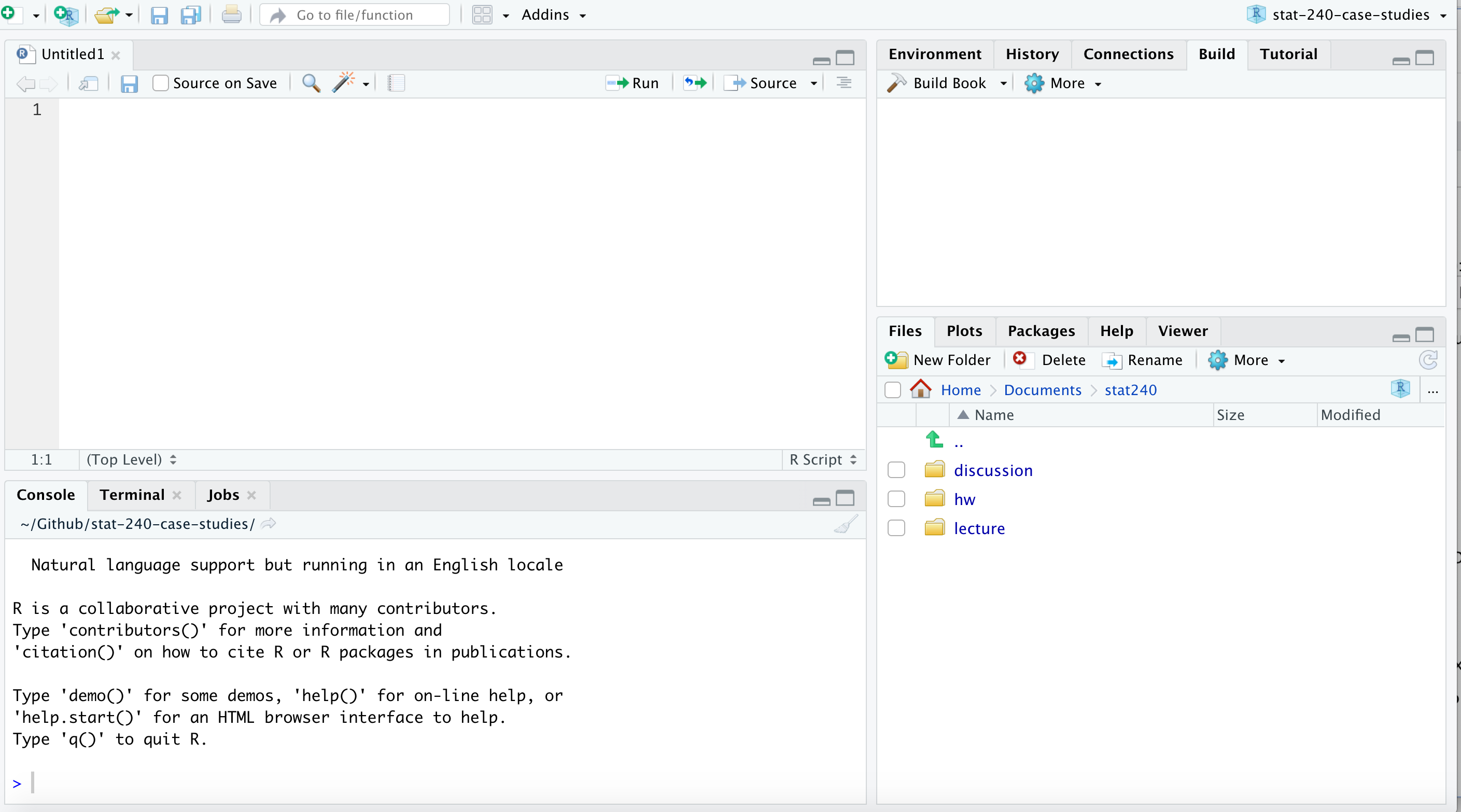
- Editor
- The upper left panel is used to edit files, such as R Markdown files.
- You can also see a spread-sheet-like view of data in a data frame here.
- There are tabs to switch among multiple files.
- Console
- You can type and execute code here directly.
- However, it is better for reproducibility to type code into a file and run the code from the file.
- We will rarely use the console
- The textbook teaches you R initially by having you type directly into the console and only later teach you about writing files.
- We aim to instill the better practice of writing code in files from the start
- Environment/History/Other stuff
- Environment shows data frames and other objects in the work space
- I never use the History tab
- File manager/Plots/Packages
- Use the Files tab to navigate your directories and find files to open
- Plots will show up here under a different tab
- Use the Packages tab to install packages
2.3 Directories (Folders)
Computers are set up to store information in a hierarchical system of directories and files. Another word for a directory is a folder, as graphical user interfaces often represent a directory with the icon of a folder like you might place into a filing cabinet. In these course notes, I will frequently use both terms.
2.3.1 The Home Directory
RStudio will designate one directory on your computer as the home directory.
- On a Mac, your home directory is something like what is below, replacing your actual account name in the obvious place.
/Users/your-account-name/
- On a Windows machine, it is the Documents folder.
Within RStudio, this is simplified to just be called Home, which you can see in the Files tab of the lower right panel.
2.4 Creating a Course Folder and Subfolders
It is best practice to create a course folder somewhere on your computer to hold all files for this course.
You might put this in Home, on your Desktop,
in your Documents folder,
in some location with all of your other courses.
Pick a place that works for you.
I might pick a folder named stat240 in my Documents folder,
such as /Users/larget/Documents/stat240/.
These course notes will assume that you have created such a folder on your computer.
The absolute path from the root directory to this course folder will likely be different for every one of us.
In the rest of these course notes,
I will refer to this course folder as COURSE
and assume that all course documents are contained within it.
2.4.1 Creating New Directories
You may certainly create new folders outside of RStudio using your operating system, but sometimes it is convenient to do so from within. Do so with the New Folder button from the Files tab in the lower right panel of the standard RStudio set up.
At this time, create your course directory.
Navigate to where you want your course folder to be, create it, and name it. Do not use spaces in the name (get into good habits).
Operating systems allow spaces in names,
but as you progress in data science,
you are likely going to need at some time in the future
to interact with files and directories from a Linux or UNIX command line, and spaces in names will make this task much more complicated than needed.
Get into the good habit of avoiding spaces in folder and file names now.
Many users replace spaces with dashes (-) or underscores (_).
Next, create several sub-directories within your course folder.
Navigate into your course folder and create some sub-folders with the names data, scripts, homework, lectures, discussion.
Later in the course, you may want others such as exams and final-project.
Each assignment in the course will start by having you download files from the Canvas course page and add them to appropriate folders and sub-folders. If you set up your sub-folders as described here, you will then be able to run code in files we provide without needing to edit and change the names of paths, directories, and folders.
2.5 Paths
Each person’s course directory will have a different path to it from Home, referred to here as COURSE.
A path is represented as a series of directory names separated by forward slashes /.
Windows actually uses back slashes, \, but within R you ought to use / and the computer will get it right regardless of your operating system.
This is important to make your code portable to other users who might be using a different operating system than yours.
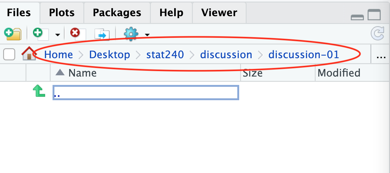
If you have a folder named discussion in your course folder with a sub-folder inside of it named discussion-01, the path to this folder is COURSE/discussion/discussion-01/.
2.5.1 Special Symbols
There are three other special symbols used in paths.
- The period
.stands for the current directory. - A double period
..stands for the parent directory, one step up from the current directory. - The tilde
~is shorthand for the home directory. (Note that this is not a dash-. The tilde~is on your keyboard as the shift character above the single backtick`, to the left of the1key.)
For me, the path ~ is the same as Users/larget.
It is useful to use the special symbol for the home directory in your code because your code can be shared with others to use on their computers without changing all of the path names.
2.6 The Working Directory
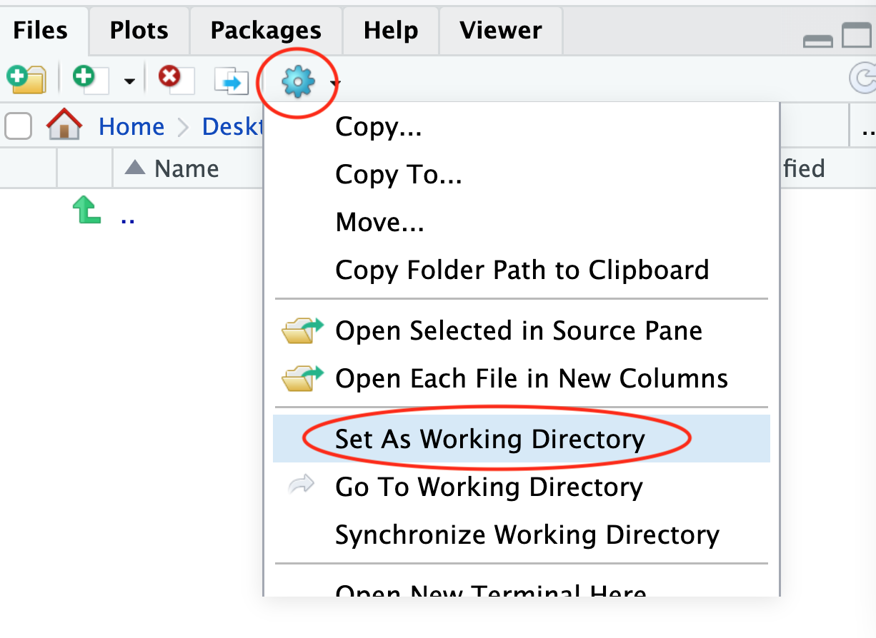
Each time you run R through RStudio, the R session is being run from one of the directories (or folders) on your computer. This directory is called the working directory. By default, your initial working directory is whatever your operating system considers to be home for you. You will want to change this each session to a folder with all of the documents for a project. For example, when working on your first discussion assignment, you will want to navigate to a folder for this assignment and then set the working directory to that folder. A quick way to set the working directory is to use the Files tab, navigate to the desired directory.
Then select Set As Working Directory from the blue settings gear icon menu of the Files tab.
Alternatively,
under the Session menu at the top of your screen,
select Set Working Directory and then one of To Source File Location or To Files Pane Location as appropriate.
2.7 Packages
There are many extensions to the R language which are distributed in packages.
In this course, we will make extensive use of the tidyverse package, which is actually a collection of many packages designed to work well together. All packages are not part of the basic R installation and need to be installed separately. While packages may be installed from the command line, I recommend using the package manager in RStudio.
2.7.1 Installing Packages
Here are the steps to install tidyverse.
- Open RStudio
- Click the Packages tab in the lower right panel
- Click the Install button
- When the dialog box opens up, type tidyverse into the Packages text box
- Make sure the Install Dependencies box is clicked (this is the default)
- Click Install
- Wait while a lot of text displays showing the status of the installation
You only need to install a package once.
It will be there the next time you open an R session.
However,
to use code from a package, you will need to use the library()
function to load the package for that session.
We will see examples of this later.
If you want some more details than what I shared above, see one of the textbooks.
- R4DS 1.4.3, https://r4ds.had.co.nz/introduction.html#the-tidyverse if you want to install the tidyverse package from the command line in the console.
2.7.2 Compilation
Sometimes, during the installation of packages, a query will arise that asks if you want to compile a package from the source code.
Do you want to install from sources the package which needs compilation? (Yes/no/cancel)
You should answer no. Answering Yes might work if your computer has already been set up to compile C, C++, and/or Fortran code, but is likely to cause an error, leading to the failure of the package to install. Just answer no each time and it will likely work for you.
Follow these instructions and install the tidyverse package now.
If you get errors when trying to install a package, reach out for help to a TA or instructor with the exact error message on Discord.
2.8 Browser Settings
In the course,
you will need to download a number of files of different types (R Markdown, PDF, CSV, HTML) from the Canvas course page and put them into specific folders.
Depending on your browser, you might need to change settings to allow this.
Some browsers will change downloaded text files by adding .txt (so that 01-discussion.Rmd becomes 01-discussion.Rmd.txt).
Some browsers will put all of your downloaded files into a Folder named Downloads without asking if you want the file somewhere different.
Some browers will automatically open a file with a program (such as using Numbers or Excel to open a .csv file).
We do not want any of these things to happen.
Here are things to check depending on which browser you are using. (If your favorite browser is not mentioned and you have figured out how to change the settings, please let me know and I will add to these instructions.)
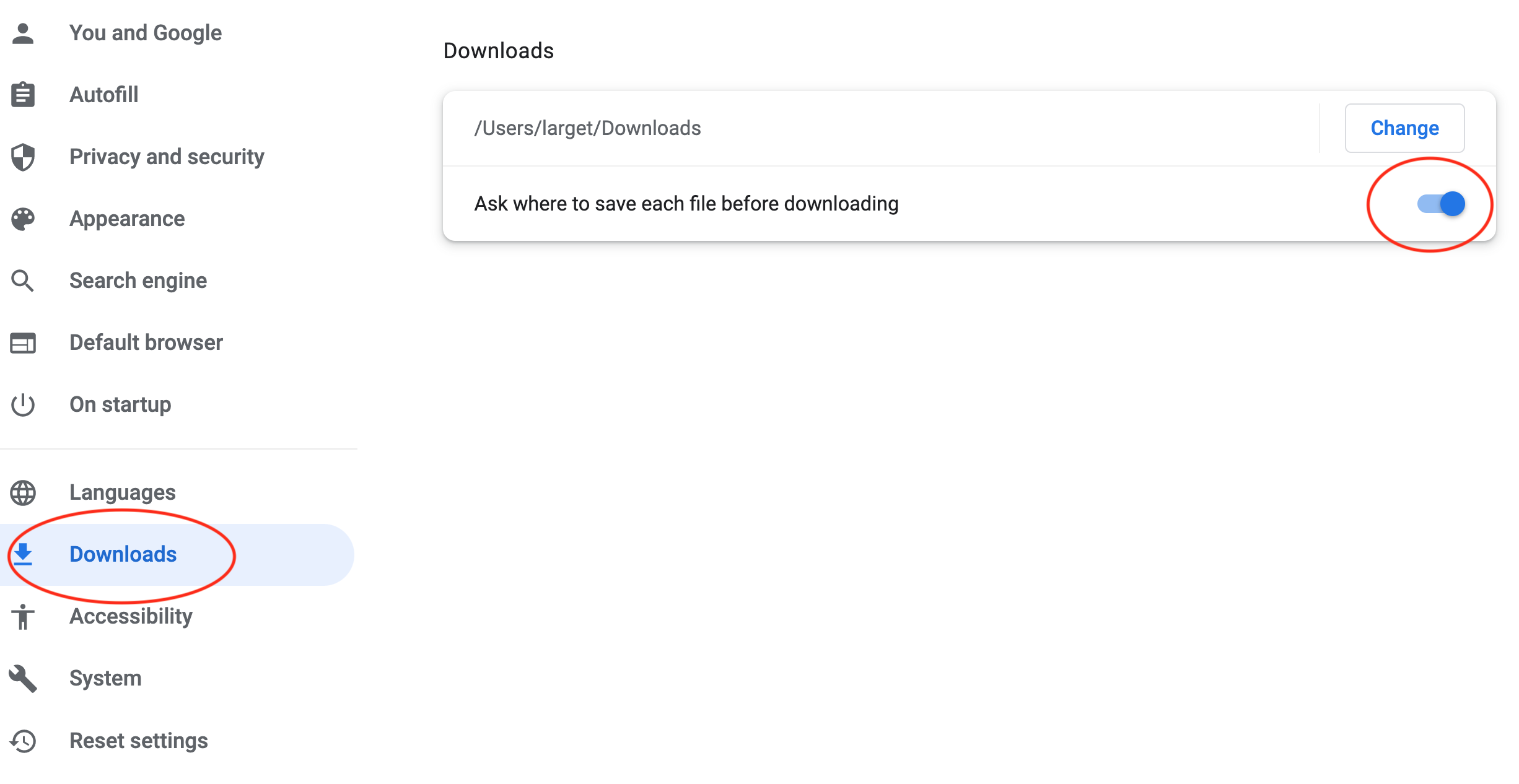
2.8.1 Chrome
- Open Chrome
- Under the Chrome menu, select “Preferences…”
- alternatively:
- click the three vertical dots under the menu bar
- click “Settings” near the bottom
- alternatively:
- Find “Downloads” in the left menu and click it
- Turn on the button “Ask where to save each file before downloading”
2.9 R Markdown Documents
In the class, you will learn to write R Markdown documents. An R Markdown document is composed of plain text, but is processed into a better formatted document, typically in HTML or PDF format. Unlike markup languages which are complicated for a human to read or interpret easily, Markdown is intentionally limited and is meant to be straightforward for a person to write, using a simple syntax for basic formatting structures such as bold and italic fonts, numbered and bullet lists, and tables. While a user has much finer control over the appearance of an output document with a markup language, Markdown’s simplicity allows the writer to focus on the primary content while still obtaining a pleasantly formatted output document with very little overhead to master a more complicated typesetting language.
R Markdown is an extension of conventional Markdown which intersperses chunks of code within the prose. Each chunk may be replaced in the final document by an object created by the code, typically a graph, other computer output, or a formatted table. The user can also display the code if desired.
R Markdown is an example of literate programming, interspersing natural language (such as English) for the writer to express thoughts with chunks of code that describe desired calculations interpretable by the computer. This concept of literate programming is very common in data science as a way for people to share their data analysis with others in a reproducible manner. It is important to learn to do this. Other platforms, such as Jupityr Notebooks, are also widely used for similar purposes, especially when using Python. In this course, each assignment will involve you editing a provided R Markdown document with your work to solve a variety of problems, followed by knitting the document into HTML for easy reading.
2.9.1 Learning R Markdown
The best way to learn R Markdown is from examples and editing provided templates rather than writing new documents from scratch. However, there is a benefit to understanding the structure of a typical document.
The beginning of most R Markdown documents is a preface called the YAML section which is separated from the rest fo the document between stand-alone lines with three dashes. YAML is a self-referencing acronym for “YAML Ain’t Markdown Language”. The material within the YAML section does not follow normal Markdown syntax and has a syntax all its own. This section is used to specify details about the document itself, such as the output format, and possibly information to construct a title page. The YAML section from the R Markdown document for John Smith’s first homework assignment might look something like this.
---
title: "Assignment 1"
author: "John Smith"
date: "6/8/2021"
output: html_document
---
The remainder of the document is a collection of text with some basic formatting syntax interspersed with chunks of code. Very frequently, the very first chunk of code will be a setup chunk which sets some options and loads libraries used later in the document. Here is an example.
```{r setup, include = FALSE}
knitr::opts_chunk$set(echo = TRUE, message = FALSE)
library(tidyverse)
```
Each chunk or R code begins with three back ticks, a left brace, and the letter r (``` {r)
followed by an optional space and chunk name (setup in the example),
followed optionally with arguments preceded by commas (, include = FALSE in the example)
and finally a right brace (}).
Chunk names are optional, but can be helpful when tracking down errors.
Be aware, however,
that all chunk names in a single document must be unique,
otherwise an error is generated when knitting.
Arguments have the structure argument-name = argument-value.
2.10 Knitting a Document
The process of turning an R Markdown document into another output format is called knitting. In RStudio, knitting is as simple as pushing a button. We will typically knit document to HTML, but knitting to PDF and Word are also possible. In a typical assignment, you start with a template R Markdown document, edit it, knit to HTML, and upload the HTML document as the solution. We often ask you to upload the .Rmd R Markdown file also so we can see your work.
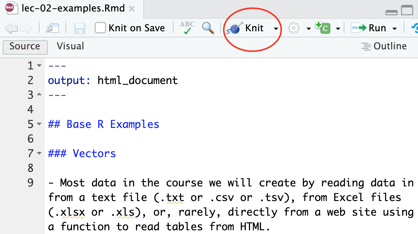
When you have an R Markdown file open in the editor,
simply click on the Knit button to knit the document into another format.
You can also click on the little downward-pointing triangle to choose the output format.
But just clicking on Knit works to create HTML when the YAML section of the document indicates that the output is an html_document.
The new file will appear in the same directory as the source file and will have the same base name as the original R Markdown file, but will have a different file extension.
For example, knitting the file lec-02-examples.Rmd process it and create the new file lec-02-examples.html.
Knitting will also open the knitted file in a separate window (using the default behavior in the RStudio preferences).
2.11 Uploading Documents to Canvas
To upload an assignment in Canvas, do the following steps.
- Open Canvas
- Click on the word Assignments from the left menu.
- Find the corresponding assignment.
- Click on the red Submit Assignment button.
- Either enter text or upload files as instructed, and then click the red Submit button.