25 Correlation and Regression
25.1 Correlation
We will use the 2019 team volleyball data to examine the relationships between quantitative variables. First, we review two key statistics to summarize a single quantiative variable. The mean \[ \bar{x} = \sum_{i=1}^n x_i \] is the balancing point of a distribution of numbers. The standard deviation, \[ s_x = \sqrt{ \frac{\sum_{i=1}^n (x_i - \bar{x})^2}{n-1} } \] is the square root of the variance and is a measure of the spread of the values around the mean. The reason that the sample standard deviation has \(n-1\) instead of \(n\) in the denominator is that if random variables \(X_1,\ldots,X_n\) are drawn from a distribution with a variance \(\sigma^2\), then \(\mathsf{E}(s_x^2) = \sigma^2\). An alternative estimator, \[ \hat{\sigma}^2 = \frac{\sum_{i=1}^n (x_i - \bar{x})^2}{n} \] is the maximum likelihood estimate of \(\sigma^2\) (for normal distributions and some others), but use of the unbiased estimator with \(n-1\) in the denominator is more common.
25.1.1 Correlation Formula
The formula for the correlation coefficient between a pair of variables \(x = (x_1,\ldots,x_n)\) and \(y = (y_1,\ldots,y_n)\) is \[ r = \frac{1}{n-1} \sum_{i=1}^n \bigg(\frac{x_i-\bar{x}}{s_x}\bigg) \bigg(\frac{y_i-\bar{y}}{s_y}\bigg) \] Note that this is (almost) the mean of the product of the z-scores of \(x\) and \(y\). We won’t prove it, but the possible values of \(r\) are \(-1 \le r \le 1\) with equality only when the points of \(x\) and \(y\) are exactly on a line (\(r=-1\) is the slope is negative, \(r=1\) if positive). The value of \(r\) is a measure of the strength and direction of a linear relationship between two quantitative variables. Two quantitative variables with a strong nonlinear relationship might have \(r\) near \(-1\), \(0\), or \(1\).
25.1.2 Correlation Examples
Here are examples of correlations from the 2019 season volleyball data using only the 14 Big 10 teams. Notice how the sign of \(r\) corresponds to the sign of the slope. When \(r\) is close to \(-1\) or \(1\), the points are more tightly clustered around the line. When \(r\) is closer to 0, there is not a strong linear trend.
big_10 = vb %>%
  filter(Conference == "Big Ten")

## Hit_pct and Opp_pct
r = big_10 %>%
  summarize(r = cor(Hit_pct,Opp_pct)) %>%
  pull(r)

ggplot(big_10, aes(x=Hit_pct, y=Opp_pct)) +
  geom_point() +
  geom_smooth(se=FALSE, method="lm") +
  ggtitle(paste("r =",round(r,3)))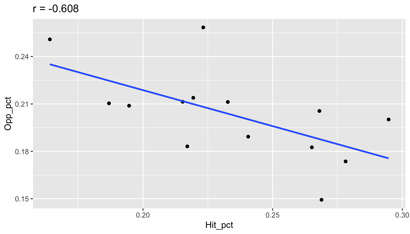
## Hit_pct and W
r = big_10 %>%
  summarize(r = cor(Hit_pct,W)) %>%
  pull(r)

ggplot(big_10, aes(x=Hit_pct, y=W)) +
  geom_point() +
  geom_smooth(se=FALSE, method="lm") +
  ggtitle(paste("r =",round(r,3)))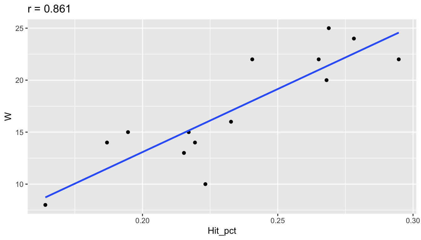
## W and L
r = big_10 %>%
  summarize(r = cor(W,L)) %>%
  pull(r)

ggplot(big_10, aes(x=W, y=L)) +
  geom_point() +
  geom_smooth(se=FALSE, method="lm") +
  ggtitle(paste("r =",round(r,3)))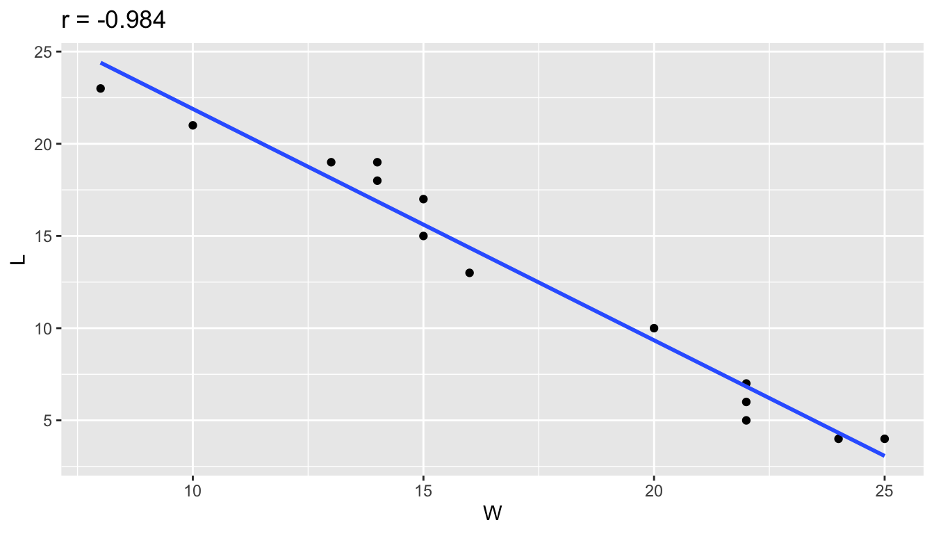
## Digs and Aces
r = big_10 %>%
  summarize(r = cor(Digs,Aces)) %>%
  pull(r)

ggplot(big_10, aes(x=Digs, y=Aces)) +
  geom_point() +
  geom_smooth(se=FALSE, method="lm") +
  ggtitle(paste("r =",round(r,3)))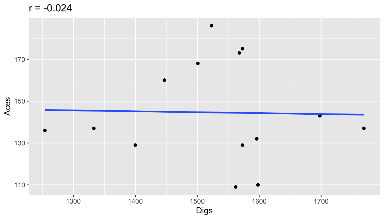
25.2 Simple Linear Regression
Correlation is a measure of relatedness between two quantitative variables.
It is symmetric, in that \(cor(x,y) = cor(y,x)\).
This is clear from the formula as changing the order of \(x\) and \(y\) just changes the order of multiplication of the z-scores, and order does not matter for multiplication of numbers.
This symmetry, however is not the case when we try to fit a model to predict \(y\) on the basis of \(x\).
As an example,
consider trying to predict the winning percentage Win_pct as a function of the averge number of kills per set.
Getting the second variable requires some data transformation.
ex1 = big_10 %>%
  mutate(kills_per_set = Kills / Sets,
         win_pct = Win_pct,
         team = Team) %>%
  select(team, kills_per_set, win_pct)

ex1
# A tibble: 14 × 3
team kills_per_set win_pct
<chr> <dbl> <dbl>
1 Illinois 13.7 0.552
2 Indiana 11.9 0.424
3 Iowa 12.6 0.323
4 Maryland 11.2 0.406
5 Michigan 14.0 0.667
6 Michigan St. 12.1 0.5
7 Minnesota 14.1 0.815
8 Nebraska 13.8 0.862
9 Northwestern 12.6 0.438
10 Ohio St. 13.5 0.469
11 Penn St. 13.7 0.857
12 Purdue 13.0 0.759
13 Rutgers 11.0 0.258
14 Wisconsin 14.5 0.786We can plot the data and add a regression line.
ggplot(ex1, aes(x=kills_per_set, y = win_pct)) +
  geom_point() +
  geom_smooth(se = FALSE, method = "lm")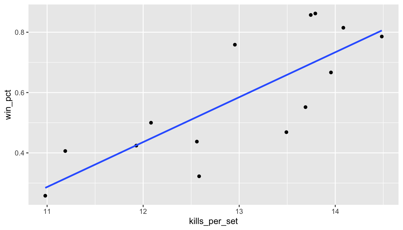
The plotted line is the least squares line, the line which minimizes the sum of squared residuals. A residual is the signed vertical distance from a point to the line, positive if the point is above the line and negative if it is below.
25.2.1 Regression Model
The model we are fitting here is \[ y_i = b_0 + b_1 x_i + \varepsilon_i \] where \(y_i\) is the winning percentage and \(x_i\) is the number of kills per set for the \(i\)th team.
The equation \(\mathsf{E}y = b_0 + b_1 x\) represents the expected value of \(y\) given \(x\). For example, we would expect a Big 10 team that averaged 13 kills per set would have a winning proportion just below 0.6, based on the graph. We see that teams with a higher number of kills per set tend to win more than teams with smaller kills per set, but the relationship is not perfect (points are not all on the line). Based on previous graphs and examining the spread of the points around the line, I would anticipate that the correlation coefficient \(r\) between these two variables would be close to 0.7 or 0.8. Let’s check.
# A tibble: 1 × 1
      r
  <dbl>
1 0.795
25.2.2 Regression Estimates
The least squares estimates are the values of \(b_0\) and \(b_1\) which minimize the following: \[ \mathsf{RSS}(b_0,b_1) = \sum_{i=1}^n (y_i - (b_0 + b_1 x_i))^2 \] The expression \(\mathsf{RSS}\) refers to residual sum of squares. We often denote \(\hat{y}_i = \hat{b}_0 + \hat{b}_1 x_i\) as the \(i\)th fitted value and the difference \(y_i - \hat{y}_i\) as the \(i\)th residual. A bit of mathematics can be used to show that the values of \(b_0\) and \(b_1\) which minimize \(\mathsf{RSS}\) are: \[ \hat{b}_1 = r \times \frac{s_y}{s_x} \] and \[ \hat{b}_0 = \bar{y} - \hat{b}_1 \bar{x} \] The slope is the correlation coefficient times the ratio of standard deviations. The intercept is the value which works so that the regression line goes through the value \((\bar{x},\bar{y})\). Here is an algebraic derivation of this to find the value of \(\hat{y}\) when \(x = \bar{x}\).
\[\begin{align} \hat{y} &= \hat{b}_0 + \hat{b}_1\bar{x} \\ &= (\bar{y} - \hat{b}_1 \bar{x}) + \hat{b}_1\bar{x} \\ &= \bar{y} \end{align}\]
25.2.3 Understanding Regression Parameters
Most times the question of interest in a regression problem involves the slope:
how does the response variable respond to changes in the explanatory variable?
On the other hand,
the intercept is the predicted value of \(y\) when the value of \(x\) is zero,
which may not be in the range of viable \(x\) values or interesting in context.
Here are the numerical estimates from our example.
We will calculate the parameters both using the formulas provided
and also using the built in function lm().
## using the formulas
ex1_sum = ex1 %>%
  summarize(mx = mean(kills_per_set),
            sx = sd(kills_per_set),
            my = mean(win_pct),
            sy = sd(win_pct),
            r = cor(kills_per_set, win_pct),
            b1 = r * sy/sx,
            b0 = my - b1*mx)
ex1_sum
# A tibble: 1 × 7
mx sx my sy r b1 b0
<dbl> <dbl> <dbl> <dbl> <dbl> <dbl> <dbl>
1 13.0 1.11 0.580 0.207 0.795 0.149 -1.35[1] -1.350161[1] 0.1488341 (Intercept) kills_per_set
-1.3501612 0.1488341 The fitted model is: \[ \text{(winning proportion)} = -1.35 + 0.149\text{(kills per set)} \]
Note that kills per set range from just under 11 to about 14.5 in this data set. The linear prediction is decent in this range of the data, but we certainly would not expect teams with 0 kills per set to win \(-135\)% of their matches.
This is an example of extrapolation. If a linear model fits all right for some range of the data \(x\), this does not imply that the linearity of the relationship will continue well outside the range of the data used to fit the model.
25.2.4 Prediction Interpretation
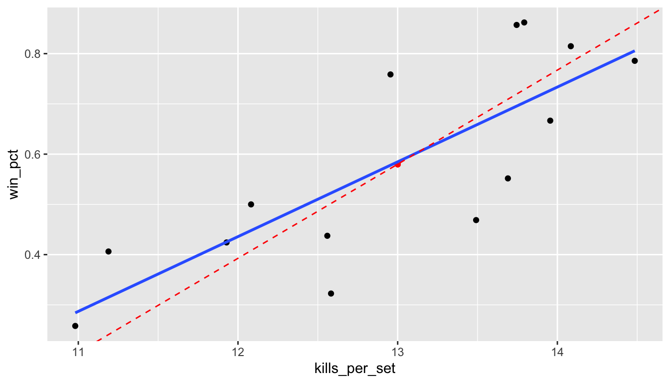
The formulas provide a way to interpret the correlation coefficient in terms of prediction. We see that a team that has 13 kills per set is expected to win 58% of their matches. If we increase the \(x\) value by \(z\) standard deviations, we expect \(y\) to change by \(rz\) standard deviations. For example, the standard deviation of \(x\) is about 1.1 kills per set. So, the predicted winning percentage of a team that has \(14.1 = 13.0 + 1 \times 1.1\) kills per set is predicted to be about \(rs_y \approx 0.8 \times 0.2 = 0.16\) larger than \(\bar{y} = 0.58\), or about 74% of the games. If \(r = 0.8\), an increase in \(x\) of 1 standard deviation corresponds to a predicted change of just 0.8 standard deviations of \(y\). This phenomenon, where the change in \(y\) is not the full number of standard deviations as the change in \(x\) is called regression toward the mean.
Here is a plot of the data again with the regression line in blue. The red dashed line also goes through the point of means \((\bar{x},\bar{y}) = (13.0,0.58)\) but has the slope \(s_y / s_x \doteq 0.187\) which is greater than the slope \(\hat{b}_1 \doteq 0.149\). The red dashed line is closer to the primary axis of the data, but will tend to overpredict \(y\) when \(x\) is larger than the mean and underpredict when \(x\) is below the mean.
25.3 Prediction of Match Outcomes
We will now use the match data to make an entirely different sort of model where we wish to use the outcomes of the matches during the season to predict the matches played during the tournament.
25.3.1 Match Data
The data I model is the scores for each set across the nearly 5,000 individidual matches between division I opponents during the 2019 women’s volleyball season. Here is the first match from this data set.
vb_matches = read_csv("data/vb-division1-2019-all-matches.csv")
vb_matches %>%
  filter(row_number() == 1) %>%
  as.data.frame() %>%
  print()
date team1 team2 site s1_1 s1_2 s1_3 s1_4 s1_5 sets_1 s2_1
1 2019-08-30 Northeastern Green Bay <NA> 16 28 25 23 NA 1 25
s2_2 s2_3 s2_4 s2_5 sets_2 winner loser attendance
1 26 27 25 NA 3 Green Bay Northeastern 210Each of the matches was on August 30, 2019. In the first match, Green Bay was the road team and beat Northeastern in four sets, 25-16, 26-28, 27-25, 25-23. Note that sets 2 and 3 went past 25 points for the winner. From this data, we can calculate that Green Bay won \(25 + 26 + 27 + 25 = 103\) points and Northeastern won \(16 + 28 + 25 + 23 = 92\) points. If we were only modeling data from this single match, we would estimate that Green Bay would win \(103/(92+103) \doteq 0.528\) of the points and Northeastern would win \(0.472\) of the points, on average, if we had them play a large number of simulated matches. To determine the probability that Green Bay would win a set, we could use simulation, and then repeat over multiple sets to estimate the probability that Green Bay would win a match.
How then, can we use the nearly 5,000 matches of data to estimate the probability that any two teams playing each other might win a hypothetical match?
25.3.2 Model
I pose a model where the strength of each team is represented by a parameter \(\theta\). The difference between the values of this parameter for two opponents (possibly with adjustments for home court and random effects) determine the chance that a team wins a point. Assume that a match is made up of a series of independent Bernoulli trials, each resulting in a point for one team or the other, until the match is won. This model assumes the chance of a team winning a point is the same whether or not the team is serving and assumes that the chance does not depend on the current score of the game. These assumptions cannot be checked using only data from the scores of each set from each match. With more detailed data (point by point summaries), w could do more.
The simple model for the probability that team \(i\) with strength \(\theta_i\) wins a single point versus team \(j\) with strength \(\theta_j\) is a function of \[ \Delta_{ij} = \theta_i - \theta_j \] where the probability is \[ \mathsf{P}(\Delta_{ij}) = \frac{1}{1 + \mathrm{e}^{-\Delta_{ij}}} \] Note that this probability is equal to \(\frac{\mathrm{e}^{\Delta_{ij}}}{1 + \mathrm{e}^{\Delta_{ij}}}\) and that the probability that team \(j\) wins the point is one minus this probability, or \(\frac{1}{1 + \mathrm{e}^{\Delta_{ij}}}\).
For more complicated models that also depend on a home-court advantage and a ramdom match effect, replace \(\Delta_{ij}\) with \(\Delta_{ij} + \alpha_{ijk} + \beta_k\) where \(\alpha_{ijk}\) is equal to \(\alpha\) if team \(i\) is home in match \(k\), \(-\alpha\) if team \(j\) is home during match \(k\) and 0 if match \(k\) is at a neutral site. The match random effect \(\beta_k\) is assumed to be drawn from a normal mean zero distribution. The simple model is an example of a logistic regression model and the complicated model is an example of a mixed effects logistic regression model.
Notice that the model requires a constraint on the values of \(\theta_i\) because adding or subtracting the same value to all \(\theta\) does not change the point probabilities. In a maximum likelihood setting, this can be accomplished by restricting the sum (or mean) of the \(\theta_i\) values to be fixed. A Bayesian approach might put a prior density on the values with mean zero and an unknown standard deviation.
25.3.2.1 The Inverse-Logistic Function
The logistic function is a function of the log odds, \(\ln(p/(1-p))\), where \(p\) is a probability. The inverse of this function is how we model the probability: \(p = \frac{1}{1 + \mathrm{e}^{-\Delta_{ij}}}\).
inv_logistic = function(x) { return ( 1/(1 + exp(-x)) )}
delta = seq(-5,5,length.out=1001)
p = inv_logistic(delta)
df = tibble(delta,p)

ggplot(df, aes(x=delta,y=p)) +
  geom_line(color="blue") +
  geom_hline(yintercept = 0) +
  geom_vline(xintercept = 0) +
  geom_hline(yintercept = 1, color="red", linetype = "dashed")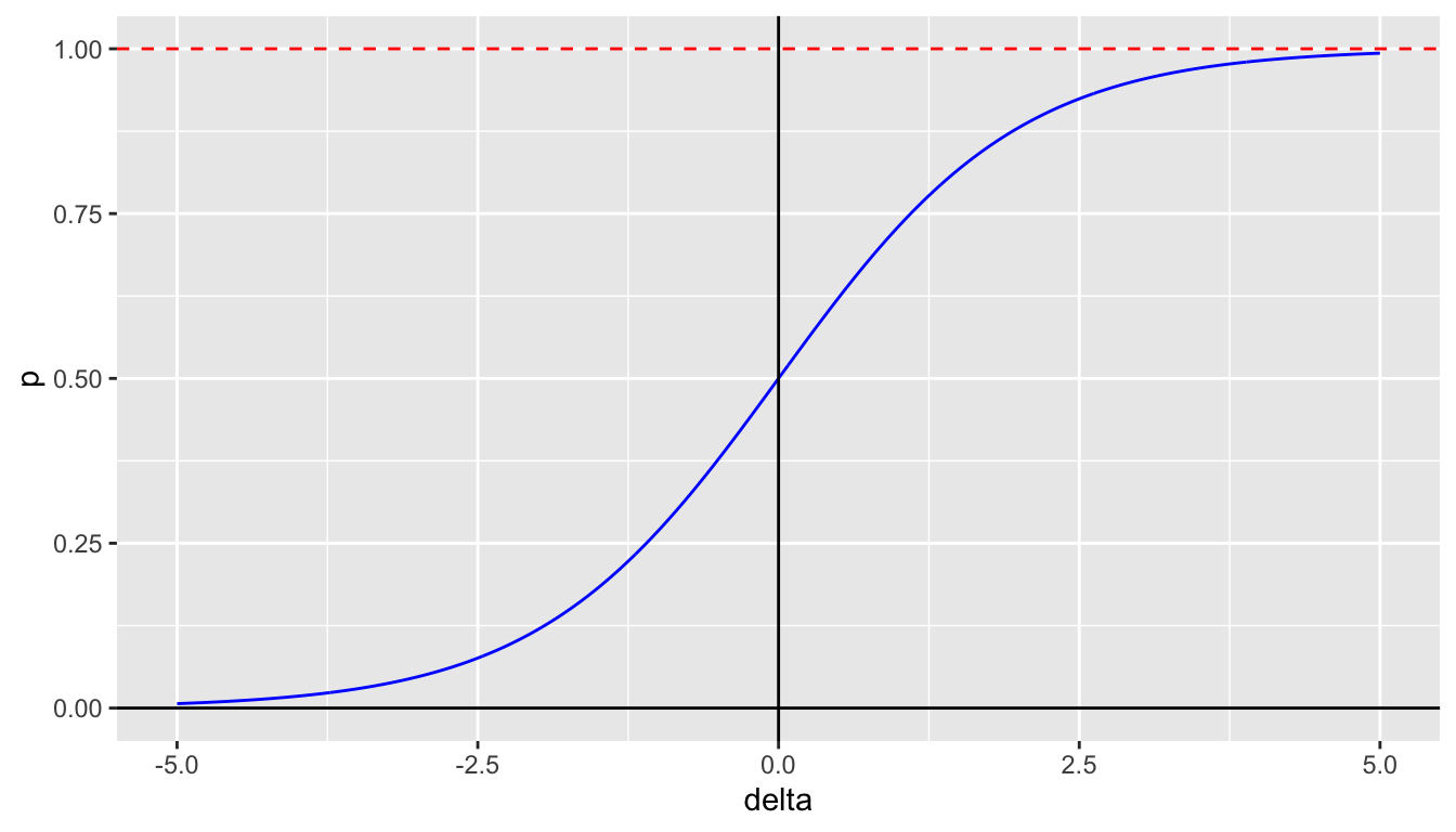
25.3.3 Likelihood
Here are results of one volleyball match.
| teams | 1 | 2 | 3 | 4 | sets |
|---|---|---|---|---|---|
| Northeastern | 16 | 28 | 25 | 23 | 1 |
| Green Bay | 25 | 26 | 27 | 25 | 3 |
This match had a total of 195 points of which team 1, Northeastern, won 92 and team 2, Green Bay, won 103. The likelihood of this result is \[ L(\Delta) = \mathsf{P}(\Delta)^{92}(1 - \mathsf{P}(\Delta))^{103} \] which achieves its maximum value when \(\mathsf{P}(\Delta) = \frac{92}{195}\), or \[ \Delta = \ln \left( \frac{92/195}{103/195}\right) = \ln \left( \frac{92}{103}\right) \doteq -0.1129 \]
Estimation with many matches is much more complicated, even in the simple model, because the same teams play multiple games against different opponents.
25.3.4 Simulation
The code in the block below can be used to simulate a set of volleyball and also a match.
The function sim_set() takes parameters delta which determines the probability a team wins and target, which is 25 for sets 1 through 4 and 15 for a set 5.
The function sim_match() simulates sets until a match is won.
inv_logistic = function(x) { return ( 1/(1 + exp(-x)) )}

sim_set = function(delta,target)
{
  p = inv_logistic(delta)
  points = c(0,0)
  repeat
  {
    pt = rbinom(1,1,p)
    if ( pt == 1 )
      points[1] = points[1] + 1
    else
      points[2] = points[2] + 1
    if ( max(points) >= target && abs(diff(points)) >= 2 )
      break
  }
  return ( points )
}

sim_match = function(delta)
{
  tab = matrix(NA,2,5)
  sets = c(0,0)
  index = 1
  repeat
  {
    if ( sum(sets) < 4 )
      result = sim_set(delta,25)
    else
      result = sim_set(delta,15)
    if ( result[1] > result[2] )
      sets[1] = sets[1] + 1
    else
      sets[2] = sets[2] + 1
    tab[,index] = result
    index = index + 1
    if ( max(sets == 3) )
      break
  }
  return ( tab )
}
This code will test the simulation to replay Northeastern, the home team, versus Green Bay, the away team, using \(\Delta = -0.113\).
set.seed(356346)

B = 10
Delta = -0.113

results = list()

for ( i in 1:B )
{
  print(i)
  results[[i]] = sim_match(Delta)
  print( results[[i]] )
  team1 = results[[i]][1,]
  team2 = results[[i]][2,]
  team1 = team1[!is.na(team1)]
  team2 = team2[!is.na(team2)]
  sets1 = sum(team1 > team2)
  sets2 = sum(team1 < team2)
  if ( sets1 > sets2 )
  {
    print(paste("Team 1 wins:", sets1, "to", sets2))
  }
  else
  {
    print(paste("Team 2 wins:", sets2, "to", sets1))
  }
}
[1] 1
[,1] [,2] [,3] [,4] [,5]
[1,] 13 25 11 24 NA
[2,] 25 21 25 26 NA
[1] "Team 2 wins: 3 to 1"
[1] 2
[,1] [,2] [,3] [,4] [,5]
[1,] 22 18 15 NA NA
[2,] 25 25 25 NA NA
[1] "Team 2 wins: 3 to 0"
[1] 3
[,1] [,2] [,3] [,4] [,5]
[1,] 12 25 17 16 NA
[2,] 25 17 25 25 NA
[1] "Team 2 wins: 3 to 1"
[1] 4
[,1] [,2] [,3] [,4] [,5]
[1,] 12 15 18 NA NA
[2,] 25 25 25 NA NA
[1] "Team 2 wins: 3 to 0"
[1] 5
[,1] [,2] [,3] [,4] [,5]
[1,] 19 25 18 22 NA
[2,] 25 19 25 25 NA
[1] "Team 2 wins: 3 to 1"
[1] 6
[,1] [,2] [,3] [,4] [,5]
[1,] 17 25 25 25 NA
[2,] 25 19 13 16 NA
[1] "Team 1 wins: 3 to 1"
[1] 7
[,1] [,2] [,3] [,4] [,5]
[1,] 20 25 23 18 NA
[2,] 25 22 25 25 NA
[1] "Team 2 wins: 3 to 1"
[1] 8
[,1] [,2] [,3] [,4] [,5]
[1,] 25 23 21 20 NA
[2,] 19 25 25 25 NA
[1] "Team 2 wins: 3 to 1"
[1] 9
[,1] [,2] [,3] [,4] [,5]
[1,] 26 27 25 NA NA
[2,] 24 25 15 NA NA
[1] "Team 1 wins: 3 to 0"
[1] 10
[,1] [,2] [,3] [,4] [,5]
[1,] 25 26 25 NA NA
[2,] 16 24 23 NA NA
[1] "Team 1 wins: 3 to 0"