19 Binomial Distributions
One of the most important discrete distribution used in statistics is the binomial distribution. This is the distribution which counts the number of heads in \(n\) independent coin tosses where each individual coin toss has the probability \(p\) of being a head. The same distribution is useful when not tossing coins, but for example, when taking random samples and counting the number of individuals in the sample that fall into a particular category. Or, if assuming that choices made by a chimpanzee in a prosocial choice experiment are independent and all have the same probability, the number of prosocial choices made.
19.1 The Binomial Probability Mass Function
The probability mass function for the binomial distribution is \[ \mathsf{P}(X=x) = \binom{n}{x} p^x(1-p)^{n-x}, \ \text{for } x=0,\ldots,n \] where \(n\) is a positive integer and \(p\) is a probability between 0 and 1.
This probability mass function uses the expression \(\binom{n}{x}\), called a binomial coefficient \[ \binom{n}{x} = \frac{n!}{x!(n-x)!} \] which counts the number of ways to choose \(x\) things from \(n\).
Example: Assume a small prosocial choice experiment with where \(n=3\) is the number of choices the chimpanzee makes and independence among the choices and let \(X\) be the number of prosocial choices made.
The collection of possible sequence from the previous chapter is
\[ \Omega = \left \{ PPP, PPS, PSP, PSS, SPP, SPS, SSP, SSS \right \} \]
\(\mathsf{P}(X=0) = \binom{3}{0} p^0(1-p)^3 = 1 \times (1-p)^3\). The sequence SSS is the only one with no prosocial choices and the probability of the specific sequence is \((1-p) \times (1-p) \times (1-p)\).
\(\mathsf{P}(X=1) = \binom{3}{1} p(1-p)^2 = 3 \times p(1-p)^2\). There are three sequence, PSS, SPS, and SPP with exactly one prosocial choice. The probability of PSS is \(p \times (1-p) \times p\), the probability of SPS is \((1-p) \times p \times (1-p)\) and the probability of SSP is \((1-p) \times (1-p) \times p\). Each of the three sequences has exactly the same probability because multiplication does not depend on the order.
\(\mathsf{P}(X=2) = \binom{3}{2} p^2(1-p) = 3 \times p^2(1-p)\). Just as the case where \(X=1\), there are three sequences and each has the same probability.
\(\mathsf{P}(X=3) = \binom{3}{3} p^3(1-p)^0 = 1 \times p^3\). The sequence PPP is the only sequence with three prosocial choices.
This example explains the format source of the binomial probability mass expression. Among all sequences of length \(n\) with \(x\) P characters and \(n-x\) S characters:
- \(\binom{n}{x}\) is the number of such sequences
- \(p^x(1-p)^{n-x}\) is the probability of any single such sequence
19.2 Mean and Variance
The mean of the binomial distribution is \(\mathsf{E}(X) = np\) and the variance is \(\mathsf{Var}(X) = n\mathsf{P}(1-p)\). These expressions can be challenging to calculate from the definitions.
\[ \mathsf{E}(X) = \sum_{x=0}^n x \binom{n}{x} p^x(1-p)^{n-x} \] \[ \mathsf{Var}(X) = \sum_{x=0}^n (x-np)^2 \binom{n}{x} p^x(1-p)^{n-x} \]
However, like in many instances, we can calculate these expectations using a method other than the definition. Here, it is most useful to recognize that the binomial random variable may be derived as the sum of \(n\) independent indicator random variables, each with probability \(p\) of being equal to 1. \[ X = I_1 + \cdots + I_n \] Note that \[ \mathsf{E}(I_i) = 0 \cdot (1-p) + 1 \cdot p = p \] for each of these indicator variables and \[ \mathsf{Var}{I_i} = (0-p)^2 (1-p) + (1-p)^2 p = p^2(1-p)+(1-p)^2p = p(1-p) \] Using the equations for expected values and variances of sums of random variables, we see that
\[ \mathsf{E}(X) = \mathsf{E}(I_1) + \cdots + \mathsf{E}(I_n) = \underbrace{p + \cdots + p}_{\text{$n$ times}} = np \]
and
\[ \mathsf{Var}(X) =\mathsf{Var}(I_1) + \cdots + \mathsf{Var}(I_n) = \underbrace{p(1-p) + \cdots + p(1-p)}_{\text{$n$ times}} = np(1-p) \]
19.3 Binomial Calculations Using R
There are several useful functions for working with the binomial distribution in R.
Each of these functions has the root binom and has as a prefix one of p, d, r, or q.
Here are examples for the \(\text{Binomial}(20,0.4)\) distribution.
19.4 Binomial Random Samples
The function rbinom() generates random binomial variables.
The first argument the number of values to generate;
the second and third arguments are the parameters \(n\) and \(p\),
but in R these have the argument names size and prob
where n is used as the number of random variables.
Here is a random sample of 5 binomial random variables. I repeat twice, once using names for the arguments and once without doing so.
[1] 8 11 10 7 5[1] 11 8 6 10 919.5 Binomial Probabilities in R
The function dbinom() measures the density, which in R for a discrete
random variable we mean the probability of individual outcomes.
You can specify multiple outcomes or just one.
 [1] 0.000037 0.000487 0.003087 0.012350 0.034991 0.074647 0.124412 0.165882
 [9] 0.179706 0.159738 0.117142 0.070995 0.035497 0.014563 0.004854 0.001294
[17] 0.000270 0.000042 0.000005 0.000000 0.000000[1] 0.1797058The function pbinom() calculate the sum of the probabilities up to the value.
So, pbinom(6,20,0.4) calculates \(\mathsf{P}(X \le 6) = \mathsf{P}(X=0) + \cdots \mathsf{P}(X=6)\).
[1] 0.2500107[1] 0.250010719.6 Binomial Quantiles
The function qbinom() locates one or more quantiles from a binomial distribution.
A value \(x\) is the p quantile of the distribution of the random variable \(X\) if both
\(\mathsf{P}(X \le x) \ge p\) and \(\mathsf{P}(X \ge x) \ge 1-p\) are true.
If \(X\) were continuous, we could simply find the value \(x\) where \(\mathsf{P}(X < x) = p\). But for discrete distributions like the binomial, a single value \(x\) might be a whole range of quantiles because probability increases in jumps.
Here is a graph of the cumulative distribution function (cdf) of the \(\text{Binomial}(20,0.4)\) distribution, \(F(x) = \mathsf{P}(X \le x)\).
The function pbinom() calculates this cdf.
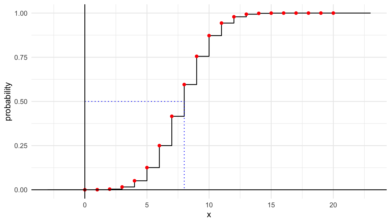
The median of the \(\text{Binomial}(20,0.4)\) distribution is the 0.5 quantile. We see this from the previous graph as the inverse of the CDF evaluated at 0.5. But 8 is also the quantile for any probability between \(\mathsf{P}(X \le 8) \approx 0.5956\) and \(\mathsf{P}(X \le 7) \approx 0.4159\).
[1] 8Note that \(\mathsf{P}(X \le 8) = 0.5956 \ge 0.5\) and \(\mathsf{P}(X \ge 8) = 0.5841 \ge 1 - 0.5\).
We can also calculate all the deciles of this distribution.
[1] 5 6 7 7 8 9 9 10 11Note that 9 is both the 0.6 and 0.7 quantiles of this distribution. Each probability \(p\) between 0 and 1 corresponds to a single quantile \(x\), one of the possible values (except if it hits the CDF exactly for some value and could be anywhere between two possible values along a horizontal step), but each possible value corresponds to a range of possible probabilities (along a vertical step).
19.7 Graphing Binomial Distributions
The file ggprob.R contains the definition of a function gbinom()
which is useful for graphing binomial distributions and
is compatible with the ggplot2 package.
There are several additional functions including geom_binom_density()
which you can use to add a binomial pdf to a plot
and functions for many other probability distributions.
Note: the function gbinom() is not part of a package and is not in base R.
You need to source the code in ggprob.R just as you do with viridis.R to be able to use the function.
Basic Usage
The first two arguments are \(n\) and \(p\).
An optional scale argument, the default of which is FALSE,
modifies the range of possible \(x\) values displayed.
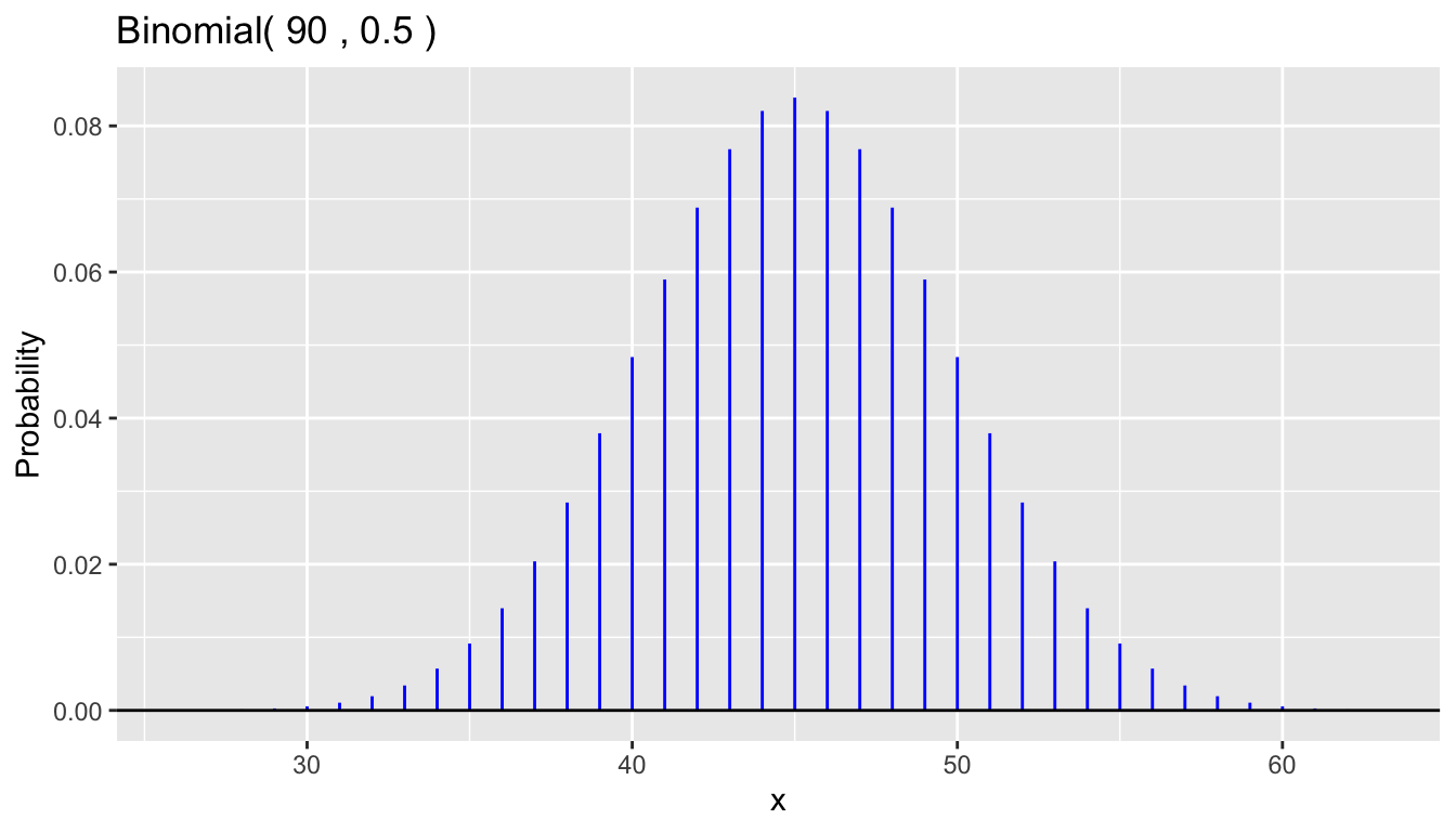
You have better control over the range of values plotted using arguments are a and b, endpoints of this interval, and color which is used for the line segments.
You can add a layer with geom_binom_density() or other ggplot2 commands.
Note that arguments to gbinom() are not aesthetics, and so need to be repeated
in geom_binom_density().
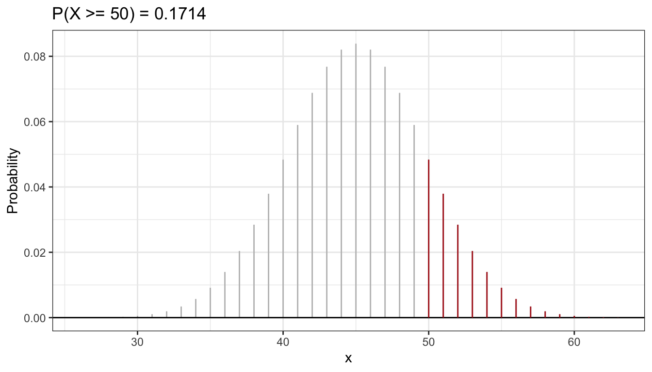
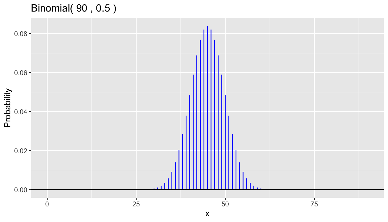
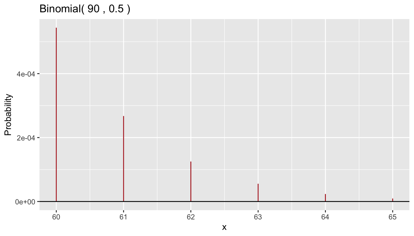
gbinom(90, 0.5, scale = TRUE, color = "gray") +
  geom_binom_density(90, 0.5, a = 50, scale = TRUE, color = "firebrick") +
  ggtitle(paste0("P(X >= 50) = ", round(1 - pbinom(49,90,0.5),4))) +
  theme_bw()