Chapter 10 Multiple regression
10.1 Formula
In a multiple linear regression there is more than one independent (input, explanatory) variable \(X\). Let the number of explanatory variables be denoted by \(k\). The explanatory variables will be denoted \(X_1\), …, \(X_k\). The \(i\)-th observation of the \(X_2\) variable will be denoted \(x_{i2}\) or \(x_{i,2}\).
The fitted multiple linear regression equation has the form:
\[\widehat{y_i} = \widehat{\beta}_0 + \widehat{\beta}_1 x_{i1} + \widehat{\beta}_2 x_{i2} + \cdots + \widehat{\beta}_k x_{ik}, \tag{10.1}\]
where \(\widehat{y_i}\) is the fitted value of the response for observation \(i\), and \(\widehat{\beta}_0\), \(\widehat{\beta}_1\), \(\ldots\), \(\widehat{\beta}_k\) are the estimated regression coefficients.
If there are two explanatory variables (\(k=2\)), the regression equation (10.1) describes a plane in 3D-space (see Figure 10.1); if there are more \(X\)s, the equation describes a hyperplane in \((k+1)\)-dimensional space.
Figure 10.1: A 3D-plot illustrating a multiple regression with two explantory variables.
10.2 Interpretation
Each regression coefficient in a multiple regression model measures the expected change in the response variable when its associated explanatory variable increases by one unit, holding all other explanatory variables constant (latin: ceteris paribus).
- Intercept (\(\widehat{\beta}_0\)):
The intercept represents the expected value of the response variable \(Y\) when all explanatory variables \(X\) equal zero. Depending on the context, this may or may not carry a meaningful interpretation.
- Slope coefficients (\(\widehat{\beta}_1, \widehat{\beta}_2, \dots, \widehat{\beta}_k\)):
The coefficient \(\hat{\beta}_j\) represents the change in the fitted response \(\hat{y}\) associated with a one-unit increase in (\(X_j\)), assuming all other (\(X\)) variables remain unchanged. This “ceteris paribus” (all else equal) interpretation distinguishes multiple regression from simple regression.
The fitted values (\(\hat{y}_i\)) lie on the regression hyperplane defined by equation (10.1). Residuals arise from deviations of the observed responses from this hyperplane.
Example:
The data were collected around 1888 from 47 French-speaking “provinces” of Switzerland. The Fertility variable is a fertility index, based on the number of children per woman, and is expressed as a percentage relative to the highly fertile Hutterite group, which serves as the benchmark. The Education variable represents the percentage of draftees with education beyond primary school. The Infant.Mortality variable indicates the percentage of live births who die before reaching one year of age.
##
## Call:
## lm(formula = Fertility ~ Education + Infant.Mortality, data = swiss)
##
## Residuals:
##      Min       1Q   Median       3Q      Max
## -15.3906  -6.0088  -0.9624   5.8808  21.0736
##
## Coefficients:
##                  Estimate Std. Error t value    Pr(>|t|)
## (Intercept)       48.8213     8.8904   5.491 0.000001875 ***
## Education         -0.8167     0.1298  -6.289 0.000000127 ***
## Infant.Mortality   1.5187     0.4287   3.543    0.000951 ***
## ---
## Signif. codes:  0 '***' 0.001 '**' 0.01 '*' 0.05 '.' 0.1 ' ' 1
##
## Residual standard error: 8.426 on 44 degrees of freedom
## Multiple R-squared:  0.5648, Adjusted R-squared:  0.545
## F-statistic: 28.55 on 2 and 44 DF,  p-value: 0.00000001126
10.3 Binary variables in linear regression
A binary variable takes only two values, typically coded as:
\[ x_{i} = \begin{cases} 1 & \text{if the characteristic is present}, \\ 0 & \text{otherwise}. \end{cases}\]
Binary variables are also called dummy variables or indicator variables. They are very common in multiple linear regression, because they allow to include categorical information – such as gender, treatment vs. control, weekend vs. weekday, yes/no, etc. – in a linear model.
Binary variables work exactly like any other regressors. For example, we have a fitted model:
\[\widehat{y}_i = \widehat{\beta}_0 + \widehat{\beta}_1 x_{i1} + \widehat{\beta}_2 d_i,\]
where \(x_{i1}\) are the values of \(X_1\) continuous variable (e.g. income) and \(d_i\) are the values of the \(X_2\) binary variable (e.g., gender = 1 if female, 0 if male).
In this model:
\(\widehat{\beta}_1\) measures the difference between predicted averages of \(Y\) when \(X_1\) increases by one unit and the value of \(X_2\) is kept constant.
\(\widehat{\beta}_2\) measures the difference between the two groups of the \(X_2\) variable after controlling for \(X_1\) (ie., keeping \(X_1\) constant).
Example:
The model describes the predictions of Right hand span based on Height and Gender using the data collected from 381 students. According to the model, when we keep gender fixed, average hand span increases by 0.08 cm (0.8 mm) with each cm of height. Controlling for height, the average difference in hand span between genders is about 1.32 cm. Typically, predicted right hand span differs from the actual value by around 1.52 cm. The model “explains” about 44.5% of the variation in hand spans.
##
## Call:
## lm(formula = right_hand_span ~ height + gender, data = a)
##
## Residuals:
##     Min      1Q  Median      3Q     Max
## -5.5086 -0.9920  0.0785  1.0021  4.2563
##
## Coefficients:
##             Estimate Std. Error t value        Pr(>|t|)
## (Intercept)  4.76530    2.11696   2.251           0.025 *
## height       0.08472    0.01253   6.759 0.0000000000527 ***
## genderMale   1.32469    0.23267   5.693 0.0000000250411 ***
## ---
## Signif. codes:  0 '***' 0.001 '**' 0.01 '*' 0.05 '.' 0.1 ' ' 1
##
## Residual standard error: 1.518 on 378 degrees of freedom
##   (2 observations deleted due to missingness)
## Multiple R-squared:  0.4449, Adjusted R-squared:  0.442
## F-statistic: 151.5 on 2 and 378 DF,  p-value: < 0.00000000000000022
10.4 Matrix notation
To present the formulas for \(\widehat{\beta}\) coefficient estimates in multiple regression, we introduce the following matrix notation:
- Design matrix \(\mathbf{X}\):
This is the matrix containing all explanatory variables. Each row corresponds to one observation, the first column consists of 1s (for the intercept), and the remaining \(k\) columns contain the observed values of the variables \(X_1, \ldots, X_k\).
- Response vector (\(\mathbf{y}\)):
A column vector containing the observed values of the response variable (\(Y\)).
Then, the formula to obtain the least-squares \(\widehat{\beta}\) vector (which is a column vector contaning the estimates \(\widehat{\beta}_0, \dots, \widehat{\beta}_k\)) is following
\[\widehat{\boldsymbol{\beta}} = (\mathbf{X}^\top \mathbf{X})^{-1}\mathbf{X}^\top \mathbf{y}\]
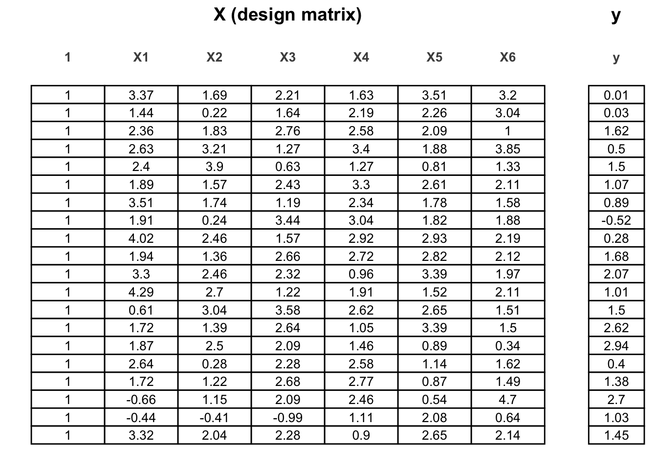
Figure 10.2: Design matrix \(\mathbf{X}\) and response vector \(\mathbf{y}\) – illustration.
10.5 Links
Multiple regression – visualization: https://istats.shinyapps.io/MultivariateRelationship/