Chapter 4 Measures of dispersion
When describing a distribution, we not only want to describe its location (using measures of central tendency), but also its dispersion (also called variability or spread).
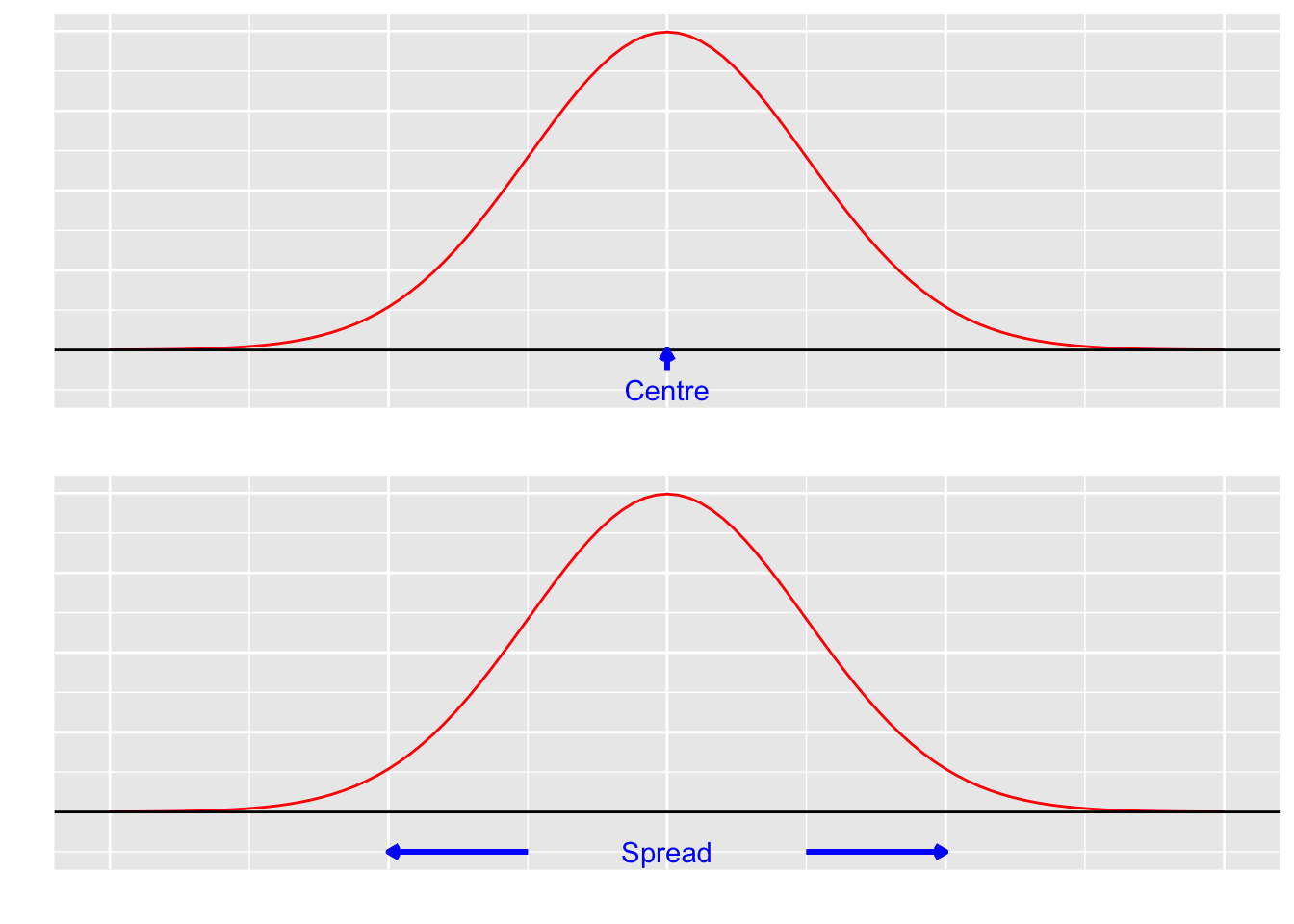
Figure 4.1: An illustration of the centre and spread of a distribution.
4.1 Standard deviation
Standard deviation is perhaps the most popular measure of the dispersion of a feature’s distribution.
The standard deviation formula appears in two versions. In this script2, we will denote them with the letters \(\widehat{\sigma}\) and \(s\), respectively.
\[\begin{equation} \widehat{\sigma}_x = \sqrt{\frac{\sum_{i=1}^n \left(x_i-\overline{x}\right)^2}{n}} \tag{4.1} \end{equation}\]
\[\begin{equation} s_x = \sqrt{\frac{\sum_{i=1}^n \left(x_i-\overline{x}\right)^2}{n-1}} \tag{4.2} \end{equation}\]
The \(X\) subscript is used in the above formulas to indicate that the standard deviation is calculated for the quantitative characteristic \(X\).
The measure \(s\) (formula (4.2)) is called the “sample” or “for-sample” standard deviation because it is usually preferred when the data being analyzed comes from a sample.
The measure \(\widehat{\sigma}\) (formula (4.1)) can also be used for a sample, but it is often called the “for-population” standard deviation. For populations, only this formula should be used. If we are dealing with a population, the “hat” over \(\sigma\) is omitted.
If you don’t know which formula to use (and there’s no one to tell you which formula they expect), use the formula (4.2).
In R, the sd() function calculates the standard deviation \(s\) using the formula (4.2). The formula for \(\widehat{\sigma}\) (4.1) is not included in standard R packages, and you must write your own function or install an additional package. The lack of a function to calculate the “sigma” formula in the standard package may provide additional clues as to which formula is typically preferred.
In spreadsheets, the standard deviation \(s\) (“for the sample”) is determined using the STDEV (STDEV) function – Google sheets, Excel or (equivalently) STDEV.S (STDEV.S) – Google sheets, Excel.
The “sigma” standard deviation (\(\widehat{\sigma}\), the formula “for the population”) can be calculated using the STDEVP function – Google Sheets, Excel or STDEV.P (STDEV.P) – Google Sheets, Excel.
Properties of the standard deviation (they are true for both \(s\) and \(\widehat{\sigma})\):
It is in the same units as the mean \(\bar{x}\) (as well as the data values \(x_i\)).
It is always non-negative: \(s \ge 0\).
If each of the values \(x_i\) is increased by the constant \(a\), the new standard deviation remains the same.
If each of the values \(x_i\) is multiplied by the constant \(k\), the new standard deviation is \(|k|\cdot s\).
4.1.1 Variance
The standard deviation is the square root of the variance. In other words, the variance is the square of the standard deviation.
There are, as you might guess, two formulas for variance:
\[\begin{equation} \widehat{\sigma}^2_x = \frac{\sum_{i=1}^n \left(x_i-\overline{x}\right)^2}{n} \tag{4.3} \end{equation}\]
\[\begin{equation} s^2_x = \frac{\sum_{i=1}^n \left(x_i-\overline{x}\right)^2}{n-1} \tag{4.4} \end{equation}\]
The variance is a “technical” measure of dispersion. Because it is based on squared differences from the mean, its unit is the square of the original unit of measurement. For example: if the data are measured in meters, the variance is measured in square meters (m²), if the data are measured in dollars, the variance is measured in dollars squared ($²). This makes variance less intuitive than the standard deviation which is the square root of variance.
Variance is always non-negative: \(s_x^2 \ge 0\).
If each of the values \(x_i\) is increased by the constant \(a\), the new variance remains the same.
If each of the values \(x_i\) is multiplied by the constant \(k\), the variance is \(k^2\cdot s_x^2\).
4.1.2 Coefficient of variation
The coefficient of variation, which is the ratio of the standard deviation to the mean, can be a better measure of variability in some situations.
Its formula for a sample is:
\[\begin{equation} V_x = \frac{s_x}{\overline{x}} \tag{4.5} \end{equation}\]
The coefficient of variation can be used for quantitative variables on a ratio scale that take exclusively (or generally) positive values.
4.1.3 Using the standard deviation
The standard deviation is a key measure of dispersion in descriptive statistics. It indicates how much individual data points differ from the mean. This measure is commonly used for purposes such as:
Comparing variability across groups, either directly or using relative measures like the coefficient of variation.
Describing approximately normally distributed variables, where two parameters — the mean and the standard deviation — are sufficient to characterize the distribution.
Calculating effect sizes, such as Cohen’s d, which expresses the standardized difference between the means of two groups.
Computing standardized scores (z-scores) to assess how far a value lies from the mean.
Detecting extreme values or outliers within a dataset.
4.1.4 The standard deviation is not the mean deviation
One might propose to measure volatility using the mean deviation, or, more precisely, the mean absolute deviation:
\[\begin{equation} MAD_x = \frac{\sum_{i=1}^n |x_i-\overline{x}|}{n} \tag{4.6} \end{equation}\]
Although both the standard deviation and the mean absolute deviation (MAD) measure dispersion, they do so in different ways. The mean deviation represents the average of the absolute differences between each observation and the mean (or median). It gives a straightforward sense of how far, on average, data points are from the center. The standard deviation, in contrast, is based on squared differences from the mean. Because of the squaring, larger deviations have a greater influence on the result. As a consequence: the standard deviation is more sensitive to extreme values than the mean deviation and it is usually larger than the MAD.
4.2 Interquartile range
Another popular measure of dispersion based on positional measures is the interquartile range (IQR):
\[\begin{equation} IQR = Q_3 - Q_1 \tag{4.7} \end{equation}\]
where \(Q_1\) is the first quartile and \(Q_3\) is the third quartile.
4.2.1 Interquartile deviation and positional coefficient of variation
Interquartile deviation and positional coefficient of variation are sometimes introduced in the Polish literature. The interquartile deviation is half the IQR:
\[ Q = IQR/2 \]
The positional coefficient of variation is the ratio of the interquartile deviation to the median:
\[ V = Q/Me \]
4.3 Boxplot
The IQR and positional measure values allow you to create a boxplot (box-and-whisker plot). This plot most often displays the median, first quartile, third quartile, as well as the minimum and maximum.
Quite often, the minimum and maximum are determined without considering outliers, which are marked separately on the chart as dots. The typical definition of an outlier in this context assumes that outliers are either less than \(Q_1 - 1.5\cdot IQR\) or greater than \(Q_3 + 1.5\cdot IQR\), although other definitions of outliers are possible.
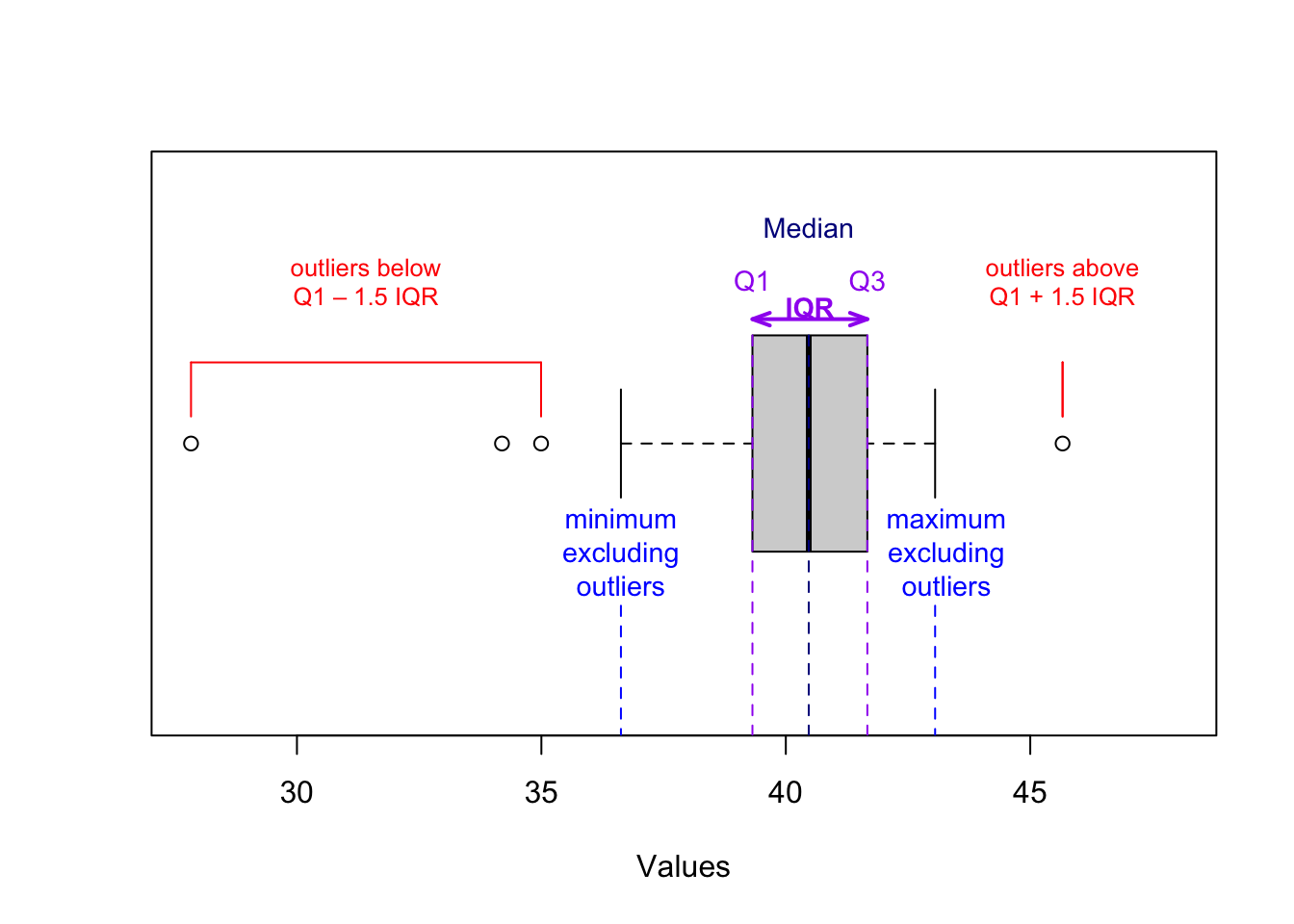
Figure 4.2: Understanding boxplots.
4.4 Links
Exploring and visualizing quantitative data - web application: https://istats.shinyapps.io/EDA_quantitative/
4.5 Discussion questions
Question 4.1 Why is the coefficient of variation an unsuitable measure for assessing the dispersion of winter temperatures in Celsius, in a Polish city?
4.6 Test questions
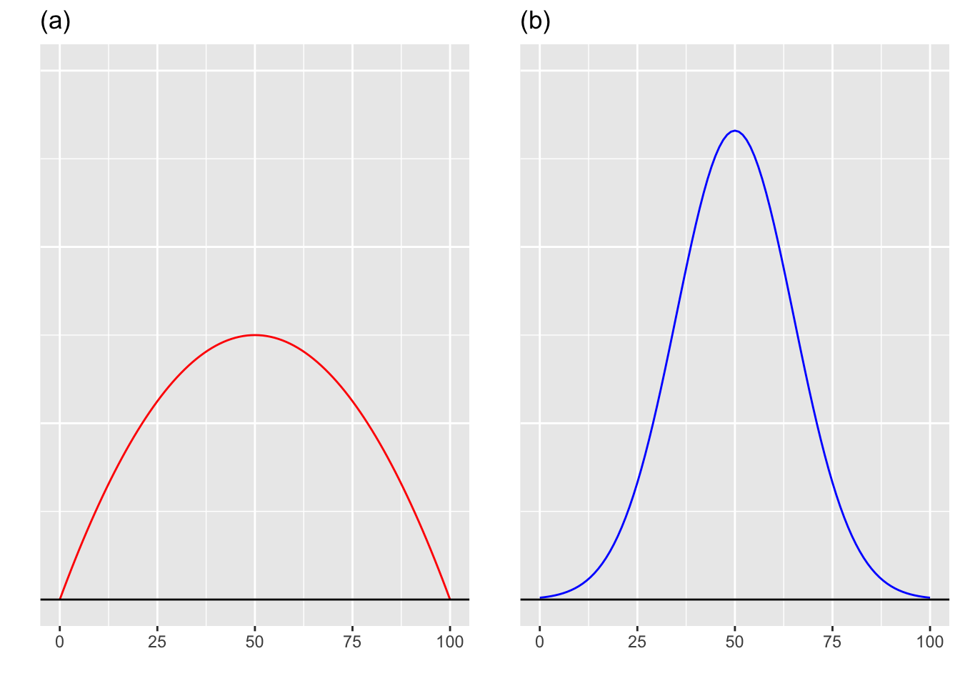
Question 4.2 (Freedman, Pisani, and Purves 2007)The two histogram sketches (density functions) are presented below. Which variable is more dispersed?
Question 4.3 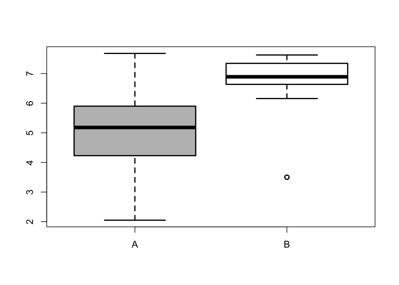
Data for groups (A) and (B) are presented in the boxplots. Which of the following is true:
Question 4.4 Match the boxplots to the corresponding histograms:
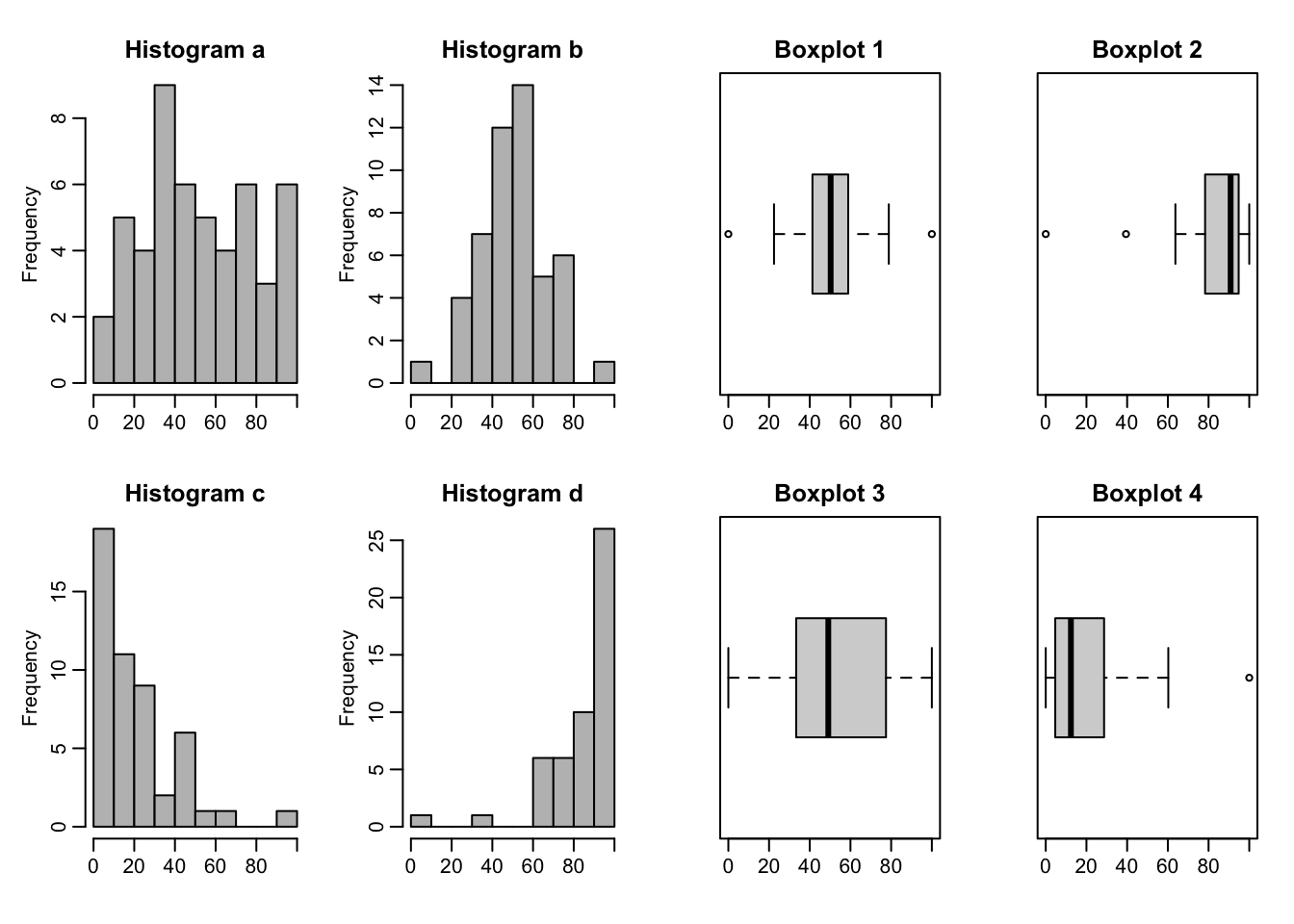
Histogram (a) Histogram (b)
Histogram (c) Histogram (d)
Question 4.5 The standard deviation (\(\widehat{\sigma}\)) of the following set of numbers: 1,2,3,4,5,6,7 is 2. What is the standard deviation of the set: 3,6,9,12,15,18,21?
4.7 Exercises
Exercise 4.1 Select one of the following sets of numbers and compute the “population” version of the standard deviation (\(\widehat{\sigma}\)) by hand. Then, verify your result using your preferred software.
1, 7, 9, 10, 13
1, 1, 11, 11, 16
1, 1, 2, 4, 7, 7, 9, 13
1, 2, 5, 6, 7, 8, 9, 10
Exercise 4.2 Select one of the following sets of numbers and calculate the sample standard deviation (\(s\)) by hand. Then, verify your result using your preferred software.
1, 7, 13, 17
1, 8, 10, 12, 14
1, 9, 10, 12, 16, 18
1, 4, 5, 6, 6, 8, 15, 19
Exercise 4.3 According to Central Statistical Office data, there are 16 towns (cities and villages) in Poland named Dobra. Based on the table below, prepare a box plot summarizing the population (number of inhabitants) of these towns.
| town or village | population |
|---|---|
| the village of Dobra in the West Pomeranian Voivodeship in Police County | 4276 |
| the village of Dobra in the Lesser Poland Voivodeship in Limanowa County | 3217 |
| the town of Dobra in the West Pomeranian Voivodeship in Łobez County | 2103 |
| the town of Dobra in the Greater Poland Voivodeship in Turek County | 1358 |
| the village of Dobra in the Lower Silesian Voivodeship in Bolesławiec County | 1115 |
| the village of Dobra in the Opole Voivodeship in Krapkowice County | 797 |
| the village of Dobra in the Łódź Voivodeship in Zgierz County | 617 |
| the village of Dobra in the Subcarpathian Voivodeship in Przeworsk County | 468 |
| the village of Dobra in the Lower Silesian Voivodeship in Oleśnica County | 364 |
| the village of Dobra in the Subcarpathian Voivodeship in Sanok County | 286 |
| the village of Dobra in Silesian Voivodeship in Zawiercie County | 276 |
| village of Dobra in Świętokrzyskie Voivodeship in Staszów County | 261 |
| village of Dobra in Łódź Voivodeship in Łask County | 246 |
| village of Dobra in Pomeranian Voivodeship in Słupsk County | 102 |
| village of Dobra in Masovian Voivodeship in Płock County | 86 |
| village of Dobra in Greater Poland Voivodeship in Poznań County | 76 |
Exercise 4.4 Create a boxplot for the order amount based on order data from an online store orders.csv.
Exercise 4.5 Graphically compare the speeds of passenger cars and motorcycles using two side-by-side boxplots. Use SpeedRadarData.csv.
Literature
Note: These are not commonly used symbols—different texts use different symbols. The formula used should be recognized from the context (often the author provides it explicitly).↩︎