Chapter 3 Central tendency and positional measures
3.1 Mean
3.1.1 Arithmetic mean
The arithmetic mean is the simplest and most basic tool for summarizing the distribution of a quantitative variable. When we simply say “mean,” or “average,” we usually mean the arithmetic mean.
The arithmetic mean of \(n\) values (labeled \(x_1\) to \(x_n\)) is:
\[\begin{equation} \overline{x} = \frac{\sum_{i=1}^n x_i}{n} \tag{3.1} \end{equation}\]
The mean can be said to be the center of gravity of a data set.
Common properties:
The sum of the deviations \((\overline{x}-x_i)\) from the mean is zero.
The arithmetic mean is a number such that the sum of the squared differences between it and each of the values \(x_i\) (i.e., the following sum: \(\sum_i(x_i-\overline{x})^2\)) is the smallest.
If each of the values \(x_i\) is increased by the constant \(a\), the new mean is \(\overline{x}+a\).
If each of the values \(x_i\) is multiplied by the constant \(k\), the new mean is \(k\overline{x}\).
3.1.2 Weighted arithmetic mean
Sometimes we assign different weights to the numbers in the described set (\(x_1\) is considered with the weight \(w_1\), \(x_2\) with the weight \(w_2\), etc.). The weights should sum to one: \(\sum_i w_i=1\). If we have weights \(w^*_i\) that do not sum to 1, they can be reduced to weights that sum to 1 using the formula \(w_i = w^*_i / \sum_i w^*_i\).
If the weights sum to 1, the arithmetic weighted average is calculated with the formula:
\[\overline{x}_{\text{weighted}} =\sum_{i=1}^n x_iw_i \tag{3.2}\]
If all weights are equal, the arithmetic weighted average is equal to the simple arithmetic average.
If our data is in the form of a discrete frequency distribution series (see 2.1.2), we can use a weighted average to determine the arithmetic mean of the data:
\[ \overline{x} =\frac{\sum_{j=1}^k x_j n_j}{n} \tag{3.3}\]
In the above formula, \(x_j\) (\(j = 1, ..., k\)) are the labels of individual values (data points), \(n_j\) is the number of occurrences of the \(j\)th value, and \(n\) is the total number of observations. The weights in this case are \(w_j = n_j/n\).
3.1.3 Harmonic mean
The harmonic mean is calculated using the following formula:
\[ H = \frac{n}{\sum_{i=1}^n\frac{1}{x_i}} \tag{3.4}\]
The harmonic mean returns a proper average in the situation when we calculate the average of quotients whose numerators are equal. For example, if I travel from location A to location B at a speed of 10 km/h and return the same route at a speed of 15 km/h, then my average travel speed will be equal to the harmonic mean of these two numbers (10 and 15), which is 12 km/h.
The formula for the weighted harmonic mean (for weights that sum to one):
\[ H_{\text{weighted}} = \frac{1}{\sum_{i=1}^n\frac{w_i}{x_i}} \tag{3.5}\]
3.1.4 Geometric mean
The geometric mean is determined based on the formula:
\[ G = \left(x_1\cdot x_2\cdot ... \cdot x_n\right)^{1/n} = \left(\prod_i x_i\right)^{1/n}\]
The geometric mean is used, among other things, to determine the average growth rate.
We can also write the formula for the geometric mean using logarithms and the exponential function: \(\text{exp}(x) = e^x\):
\[ G = \text{exp} \left(\frac {1}{n}\sum \limits _{i=1}^{n}\ln x_{i}\right) \tag{3.6}\]
It is also possible to calculate a weighted geometric mean (the weights \(w_i\) sum to one):
\[ G = \text{exp} \left(\sum \limits _{i=1}^{n}w_i\ln x_{i}\right) \tag{3.7}\]
3.2 Median
The median divides a given set (sample, population) into two equal parts. If we sort a set of numbers, the median will be the middle value or, if there is no single middle observation, the arithmetic mean of the two middle values.
The median is less sensitive to outliers than the arithmetic mean, and therefore better describes the central tendency (average value) in a set with significant extremes and/or an asymmetric distribution of values.
It is not necessary to know all the values to determine the median. This can be important in survival analysis (e.g., when measuring the lifespan of a product or customer).
The median is less convenient than the arithmetic mean in mathematical calculations. The arithmetic mean is usually preferred (“better” than the median) for statistical inference, for example, when we want to understand the distribution of a population based on a random sample. Calculating the median typically requires more processing power and computer memory.
3.2.1 Approximating the median from a grouped frequency distribution
If we have a grouped interval frequency distribution table (i.e., data grouped into class intervals with counts), the median cannot be obtained “exactly”. It may be approximated by linear interpolation. In such a situation, the following formula can be used:
\[ Me = l_M + \left(\frac{n}{2}-n_{M-}\right)\frac{h_M}{n_M} \tag{3.8}\] where:
\(n\) is the frequency of the analyzed population,
\(n_M\) is the frequency of the median interval (the interval containing the median),
\(h_M\) is the width of the median interval,
\(l_M\) is the lower bound of the median interval,
\(n_{M-}\) is the cumulative frequency of all intervals below the median interval.
It is worth remembering that using this formula implicitly assumes a uniform distribution of values within the class interval.
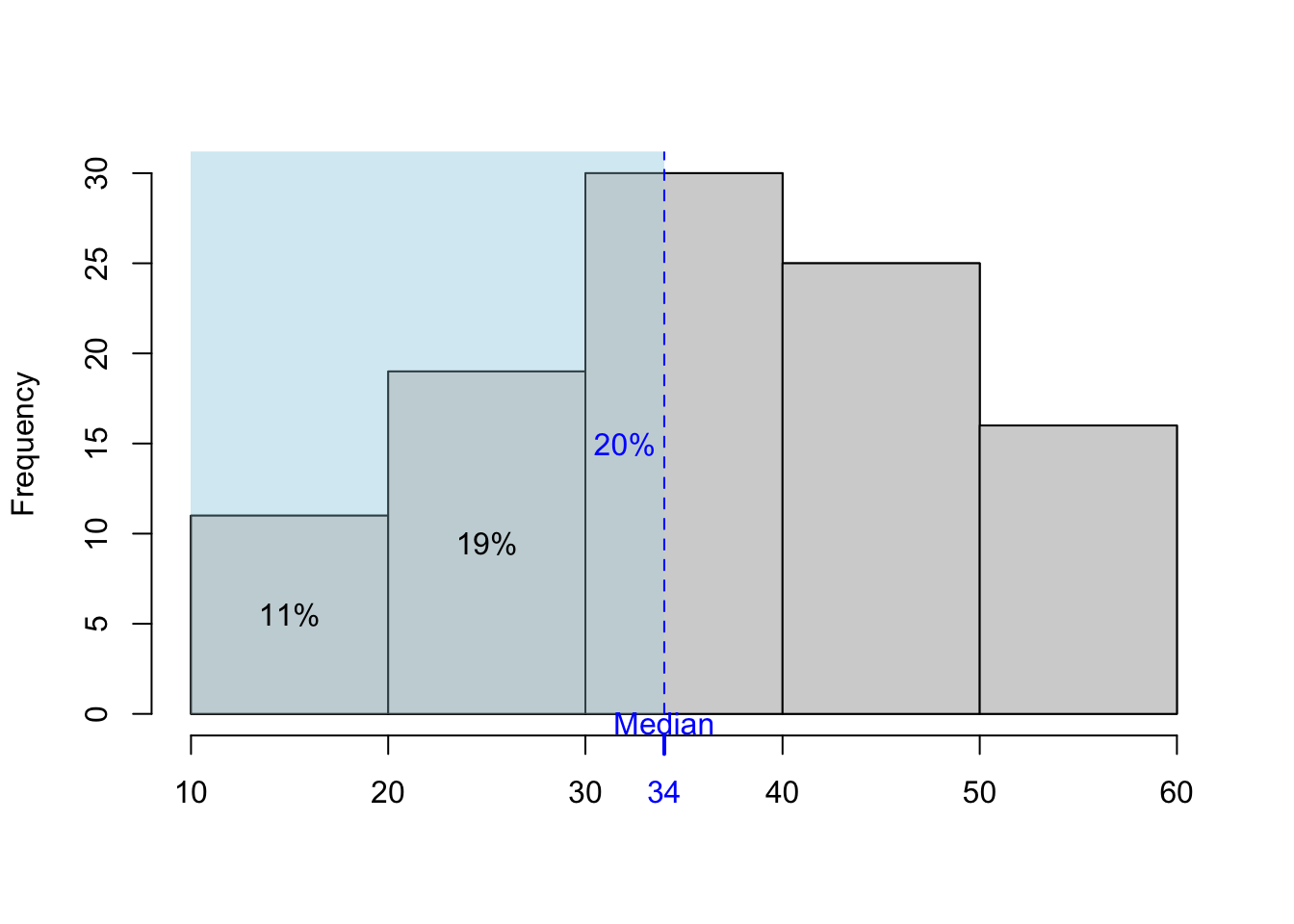
Figure 3.1: Approximating median from the grouped frequencies – illustration.
3.3 Mode
The mode is the value that occurs most frequently in a data set (a series of numbers). A series can have multiple modes. Mode can be determined for quantitative and qualitative variables.
3.3.1 Determining the mode from an interval distribution series
If the numbers refer to a continuous feature, this definition of mode is no longer valid. In such situations, a different definition of mode is often used: it is the location on the X-axis for which the histogram (created from the grouped frequency distribution table) peaks. In such a situation, the mode depends on how the data are grouped into classes and on the precise method of determining the location on the X-axis (the midpoint of the interval or interpolation).
The interpolation formula for determining the mode is:
\[ Mo = l_m + \frac{n_m - n_{m-1}}{(n_m - n_{m-1}) + (n_m - n_{m+1})} \cdot h \tag{3.9}\]
where:
\(l_m\) is the lower bound of the modal (dominant) interval, i.e., the one whose frequency \(n_m\) is the largest,
\(n_m\) is the frequency of the modal interval,
\(n_{m-1}\) is the frequency of the interval preceding the modal interval,
\(n_{m+1}\) is the frequency of the interval following the modal interval,
\(h\) is the width of the intervals.
The above formula assumes that all widths of the \(h\) intervals are equal. If they are not equal, it is necessary to determine the density \(d_j=n_j/h_j\) in each interval \(j=1,2,3,...,k\). In this situation, the formula is:
\[ Mo = l_m + \frac{d_m - d_{m-1}}{(d_m - d_{m-1}) + (d_m - d_{m+1})} \cdot h_m \tag{3.10}\]
where:
\(l_m\) is the lower bound of the modal (dominant) interval, i.e., the one whose frequency density \(d_m=n_m/h_m\) is the highest,
\(d_m\) is the frequency density of the modal interval,
\(d_{m-1}=n_{m-1}/h_{m-1}\) is the frequency density of the interval preceding the modal interval,
\(d_{m+1}=n_{m+1}/h_{m+1}\) is the frequency density of the interval following the modal interval,
\(h_m\) is the width of the modal interval.
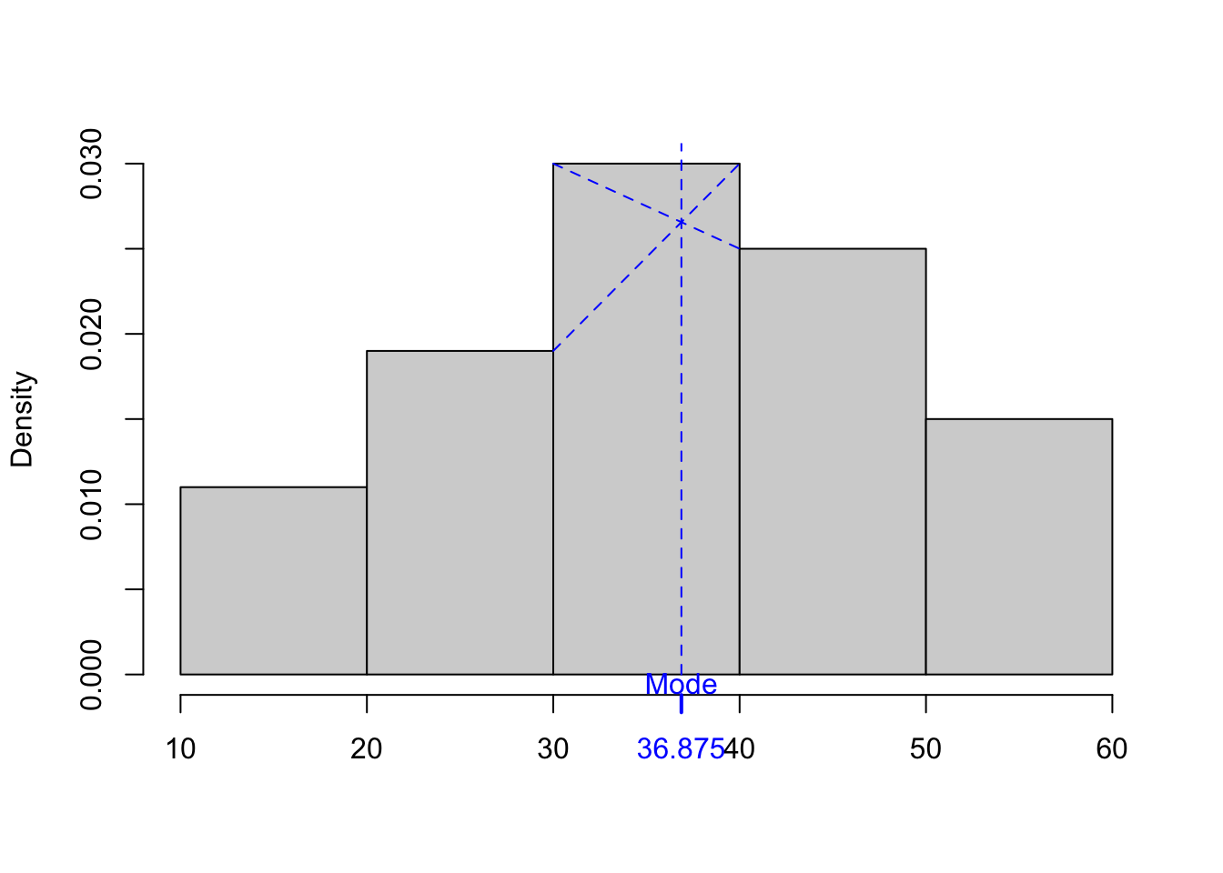
Figure 3.2: Approximating mode from the grouped frequencies – illustration.
3.3.2 Relationship between mode, median, and mean
If the data is (close to) symmetrical and unimodal, all three are (approximately) equal.
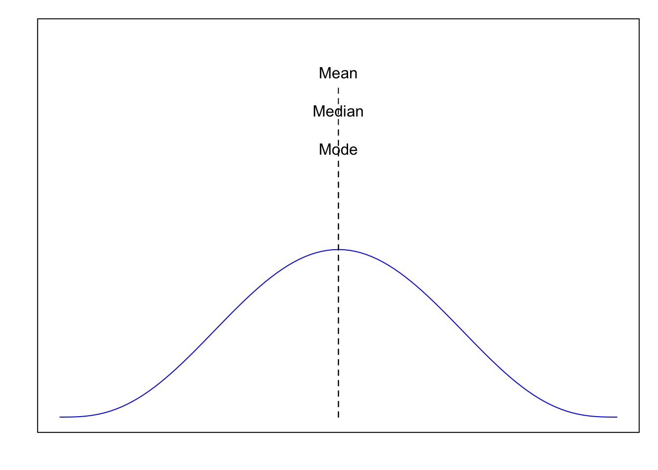
Figure 3.3: Mode = Median = Mean for a symmetrical unimodal distrtibution.
If the distribution is positively skewed (right-skewed), often – but not always – Mode < Median < Mean. The tail on the right „pulls the mean higher”.
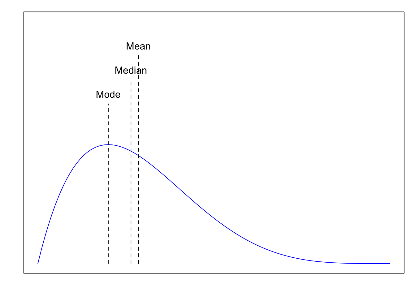
Figure 3.4: Illustration of Mode < Median < Mean for the positively skewed distrtibution.
If the distribution is negatively skewed (left-skewed), often – but not always – Mean < Median < Mode. The tail on the left „pulls the mean lower”.
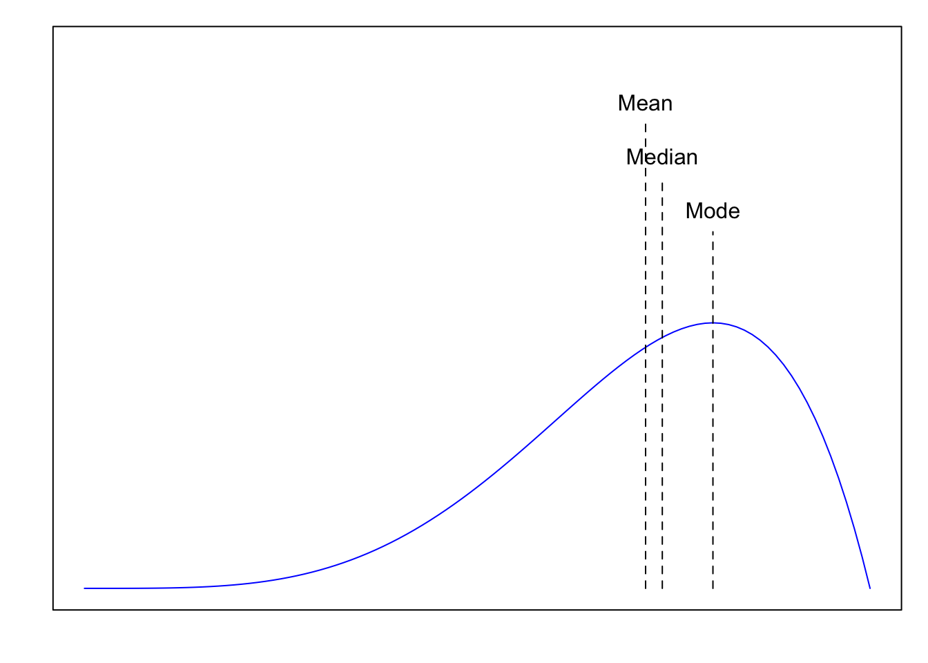
Figure 3.5: Illustration of Mean < Median < Mode for the negatively skewed distrtibution.
3.4 Quantiles
Quantiles are measures based on an ordered (sorted) data set. An example of such a measure is the most well-known quantile: the median.
3.4.1 Quartiles
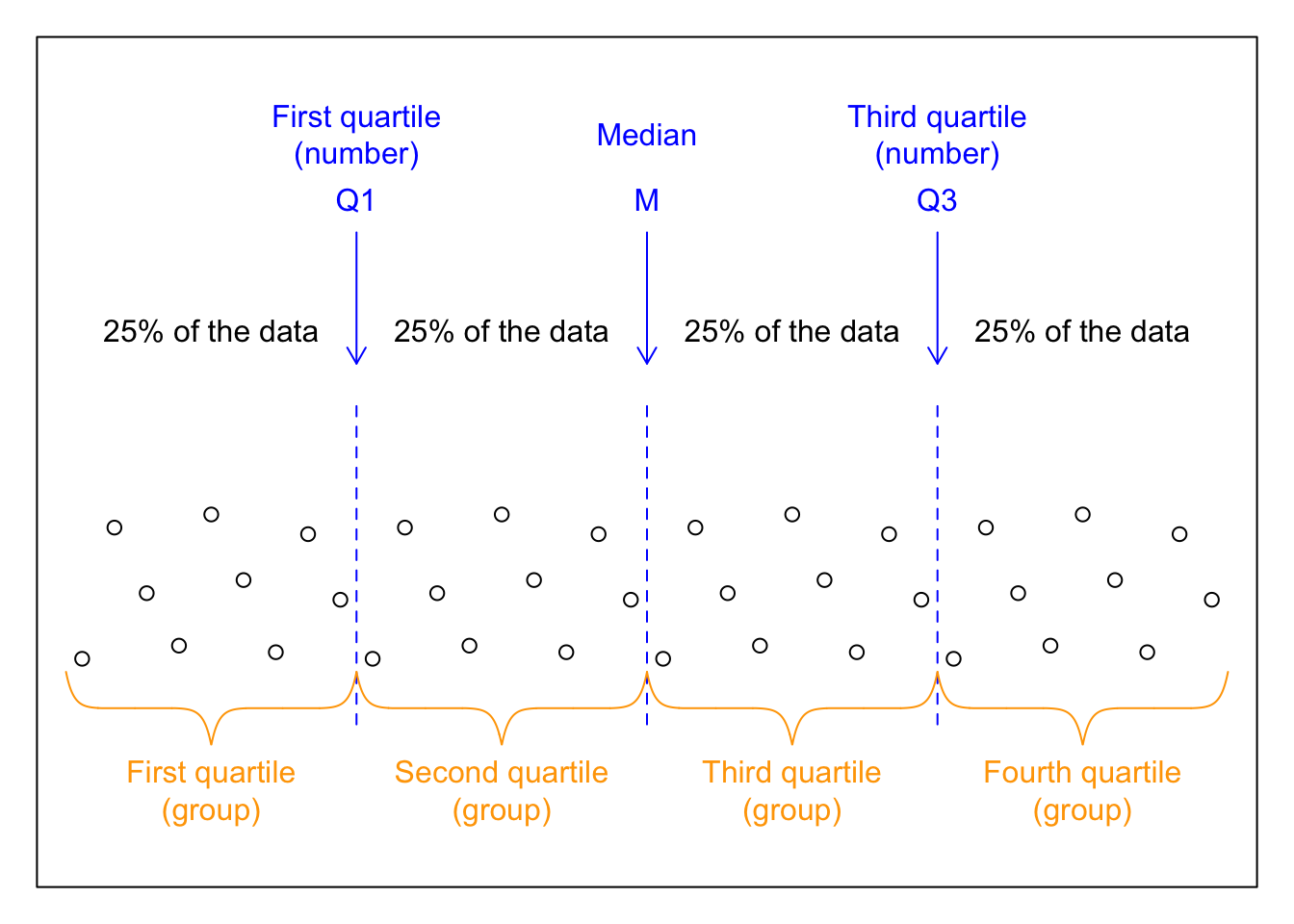
The median divides a given set (sample, population) into two equal parts. Quartiles (first, second = median, and third) divide the set into four equal parts.
The first (lower) quartile is (in the first sense, see below) the number that divides the data set into the bottom 25% of observations and the top 75% of observations.
The second quartile is the median. It divides the data set into the bottom 50% and the top 50%.
The third (upper) quartile is the number that divides the data set into the bottom 75% of observations and the top 25%.
3.4.2 Two meanings of the word quartile
It’s worth noting that the word quartile__ (like the words for some other quantiles, such as quintile or decile) can have two meanings:
in the first meaning, a quartile (quintile, decile) is a numerical value separating a specific fraction (e.g., the first quartile separates the bottom 25%).
in the second meaning, a quartile refers to observations that fall into a specific quarter with respect to the characteristic being analyzed. To avoid ambiguity, the term “quartile group” can be used.
For example, consider household disposable income. The second quartile is:
in the first meaning – the median income,
in the second meaning – those households whose income falls between the first quartile (in the first meaning) and the median.
3.4.3 Quintiles
Quintiles divide the data set into 5 groups. For example, the second quintile (in the first sense) divides the data set into the bottom 40% and the top 60%.
3.4.4 Deciles
Deciles divide the data set into 10 groups. For example, the 3rd decile divides the data set into the bottom 30% and the top 70%.
3.4.5 Percentiles
Percentiles or percentiles divide the data set into 100 groups. It is assumed that fractional percentiles can be defined analogously, e.g., the 97.5th percentile divides the data set into the bottom 97.5% and the top 2.5%.
Figure 3.6: Popular types of quantiles
3.4.6 Determining Quantiles in Practice
In practice, it turns out that the definition presented above is not sufficiently clear. For example, is it possible to determine the first quartile for a data set consisting of only 11 observations based on the general definition?
The table below shows the calculation of quartiles for a simple data set consisting of ten numbers: 1, 1, 2, 2, 4, 5, 6, 7, 9, 10, using nine (!) algorithms implemented in R.
Without delving into the intricacies of the algorithms, it’s worth noting that R and Excel/Google (the QUARTILE function) use algorithm 7 by default.
| Algorithm number | Quartile 1 | Median | Quartile 3 |
|---|---|---|---|
| type = 1 | 2.000000 | 4.0 | 7.000000 |
| type = 2 | 2.000000 | 4.5 | 7.000000 |
| type = 3 | 1.000000 | 4.0 | 7.000000 |
| type = 4 | 1.500000 | 4.0 | 6.500000 |
| type = 5 | 2.000000 | 4.5 | 7.000000 |
| type = 6 | 1.750000 | 4.5 | 7.500000 |
| type = 7 | 2.000000 | 4.5 | 6.750000 |
| type = 8 | 1.916667 | 4.5 | 7.166667 |
| type = 9 | 1.937500 | 4.5 | 7.125000 |
3.5 Links
Mean as the balance point visualization: https://www.geogebra.org/m/y4peqgpk
Mean vs. Median - Web App: https://istats.shinyapps.io/MeanvsMedian/
Distribution Asymmetry vs. Mean and Median - Simulation: https://college.cengage.com/nextbook/statistics/utts_13540/student/html/simulation2_3.html
Examples of percentile grids from the WHO: https://www.who.int/tools/child-growth-standards/standards/weight-for-age
Examples of percentile grids from the Polish Institute of Mother and Child: https://i.wp.pl/a/i/szkola2/pdf/siatki_centylowe.pdf
Geometric mean – facebook reel: https://www.facebook.com/reel/1304267144759969/?fs=e&s=TIeQ9V&fs=e&fs=e
Harmonic mean – facebook reel: https://www.facebook.com/share/v/1CxaLRxjJo/?mibextid=wwXIfr
3.6 Discussion questions
Question 3.1 Can a qualitative variable have a mode? Give an example.
Question 3.2 Can a qualitative variable have a median? Provide an example of the type of variable for which a median can be determined.
3.7 Exercises
Exercise 3.1 The following observations are given:
\[x_1 = 2,\; x_2 = 4,\; x_3 = 1,\; x_4 = 3,\; x_5 = 5,\; x_6 = 2,\; x_7 = 4\]
Calculate:
\(\displaystyle \sum_{i=1}^{7} x_i\:\:\:\:\:\) =
\(\displaystyle \overline{x} =\frac{1}{7}\sum_{i=1}^7 x_i\:\:\:\:\:\) =
\(\displaystyle \sum_{i=1}^{7} x_i^2\:\:\:\:\:\) =
\(\displaystyle \sum_{i=1}^{5} x_i\:\:\:\:\:\) =
\(\displaystyle \sum_{i=1}^{7} (x_i - \overline{x})\:\:\:\:\:\) =
\(\displaystyle \frac{1}{7}\sum_{i=1}^7 x_i+2 \quad\) =
\(\displaystyle \prod_{i=1}^{7} x_i\quad\) =
\(\displaystyle \sum_{i=1}^{7} i\quad\) =
\(\displaystyle \prod_{i=1}^{7} i\quad\) =
Exercise 3.2 (Freedman, Pisani, and Purves 2007)Which of the following two lists has a bigger average? Or are they the same? Try to answer without doing any calculations.
List A: 5, 4, 6, 9, 8
List B: 5, 4, 6, 9, 8, 10
Exercise 3.3 (Freedman, Pisani, and Purves 2007)
Ten people in a room have an average height of 166 cm. An 11th person, who is 199 cm tall, enters the room. Find the average height of all 11 people. cm
Twenty-one people in a room have an average height of 166 cm. A 22nd person, who is 199 cm tall, enters the room. Find the average height of all 22 people. cm
Twenty-one people in a room have an average height of 166 cm. A 22nd person, enters the room. How tall would he/she have to be to raise the average height by 3 cm? cm
Exercise 3.4
We drove at 60 km/h for an hour, then 120 km/h for another hour. What was our average speed?
We drove at 60 km/h for 100 km, then 120 km/h for 100 km. What was our average speed?
We drove at 60 km/h for 60% of the time (e.g., 3 out of 5 hours), and at 120 km/h for 40% of the time (e.g., 2 out of 5 hours). What was our average speed?
For 60% of the distance (e.g., 300 km), we traveled at 60 km/h, and for 40% of the distance (e.g., 200 km), we traveled at 120 km/h. What was the average speed?
Exercise 3.5 Based on the order data from the online store (orders.csv), calculate and interpret the median order amount, first quartile, third quartile, the IQR, tenth percentile, and ninetieth percentile.
Exercise 3.6 Based on the radar data (SpeedRadarData.csv), calculate and interpret the median, lower, and upper quartiles for
two-wheelers,
passenger cars.
What could be the reason for the differences?