Chapter 1 Statistical data

1.1 Observational studies and experiments

Where do data come from? In statistics, it is often important to distinguish two main ways of collecting data: observational studies and experiments.

Experiments occur when the researcher can decide on certain variables (treatments) and measure the response to a given treatment. Experiments make it easier to identify cause-and-effect relationships.

Observational studies occur when the researcher has no control over the variables but simply records reality. In this situation, it is much harder (and without strong additional assumptions, impossible) to establish causal relationships. If certain variables and potential responses are linked, we speak of correlation, association, or statistical dependence.

1.2 Population and sample

A population refers to the entire set of units, objects, or phenomena under study. It may be finite (e.g., all students in a given school) or very large, even theoretically infinite (e.g., all dice rolls, all potential patients with a given disease).

A sample is a subset of the population that is actually studied and on the basis of which we draw conclusions about the population.

Example:

Population: all residents of Poland.
Sample: 1,000 people randomly selected to take part in a survey.

In practice, we usually have a sample, even though the population is what we are theoretically interested in. Statistical inference refers to methods that allow us to draw conclusions about a population based on a sample.

1.3 Sources of statistical data

There are many ways to collect data, for example:

Survey/questionnaire data – information provided directly by the respondent.
Researcher-collected data – field notes, recordings, lab tests, clinical trials.
Automatically collected data – sensor data (e.g., Internet of Things, satellites, smart bands), transactional data (sales records, banking logs, online activity).
Textual and multimedia data – documents, social media, images, video, audio.

It is also important to note that primary data may later be processed and reused for different purposes. From this perspective, we can distinguish:

Primary data – collected and used for a specific purpose.
Secondary data – previously collected by others, then reused and processed (e.g., official statistics, company reports, administrative registers).
Sometimes, tertiary data data, ie. compilations and syntheses (e.g., encyclopedias, meta-analyses) are mentioned as well.

1.4 Quantitative and qualitative variables

Two fundamental types of statistical variables are:

quantitative (numeric, metric) variables and
qualitative (categorical) variables.

Quantitative variables take numerical values. Mathematically, they can be further divided into discrete variables (taking distinct values, e.g., number of children) and continuous variables (taking any value within an interval, e.g., call duration, proportion of people wearing glasses).¹

Qualitative variables take non-numeric values. They remain qualitative even if recorded with digits (e.g., dog breed is a qualitative variable even if we assign numbers to breeds).

1.5 Measurement scales

1.5.1 Four main scales of measurement

A useful classification of variables is based on measurement scales:

Qualitative variables use the nominal i ordinal scale.

Quantitative variables use the interval and ratio.

Nominal variables are categorical variables whose values have no inherent order (e.g., blodd type, religion, dog breed).

Ordinal variables are categorical variables with a meaningful order (e.g., education level or Likert scale responses).

Interval variables are numeric variables where differences are meaningful, but ratios are not (e.g., Celsius temperature, calendar year of birth). It is often said that for these variables, the zero point is set arbitrarily — the arbitrariness of zero is indeed a useful way to identify variables on an interval scale.

Ratio variables are numeric variables where both differences and ratios are meaningful (e.g., number of cars owned, price, height).

1.5.2 Why measurement scales matter

Measurement scales determine which statistical tools and measures can be applied. For example:

Mean, standard deviation, skewness → only for quantitative variables.
Coefficient of variation → meaningful only for ratio variables.
Median and other quantiles → for quantitative and ordinal variables.
Mode → can be determined for all types of variables, even nominal.
Pearson correlation → for quantitative variables (with binary variables as a special case).
Spearman rank correlation → for ordinal and quantitative variables.
Histogram → for grouped quantitative variables (though once grouped, the data become ordinal).
Scatterplot → for pairs of quantitative variables.
Regression explanatory variables → quantitative and binary variables.
Ranks → for quantitative and ordinal variables.

1.5.3 Other scales

Some variables do not fit neatly into the four basic categories. Two common special cases are:

Binary (dichotomous) variables: two possible values, often coded 0/1 (e.g., Yes/No). These are technically qualitative but often treated like quantitative variables.

Cyclic scales: values repeat in cycles (e.g., months of the year, days of the week, hours of the day, compass directions, angles).

1.6 Other data classifications

By time dimension:

Cross-sectional data – collected at one point in time (snapshot).
Time series data – repeated measurements at regular time intervals.
Panel/longitudinal data – tracking the same units over time (a mix of cross-sectional and time series).

By structure/format:

Structured data – organized in tables, relational databases.
Unstructured data – texts, images, audio, video, raw logs.
Semi-structured data – partially organized (e.g., JSON, XML, web logs).

By other features:

By granularity – individual-level vs. aggregated data.

By spatial dimension – with or without a spatial dimension (e.g., GIS data).

By domain – e.g., medical, financial, or general-purpose data.

1.7 Numbers

1.7.1 Names: short and long scale

Be careful when translating large number names between languages (Polish, English, Ukrainian, etc.). Even Google Translate may make mistakes.

pol. miliard = eng. billion

pol. bilion = eng. trillion

pol. biliard = eng. quadrillion

pol. trylion = eng. quintillion

Table 1.1: Names of large numbers
Number	Polish	English	Ukrainian
1 000 000	milion	million	мільйон
1 000 000 000	miliard	billion	мільярд
1 000 000 000 000	bilion	trillion	трильйон
1 000 000 000 000 000	biliard	quadrillion	квадрильйон
1 000 000 000 000 000 000	trylion	quintillion	квінтильйон

1.7.2 Decimal symbol and thousands separator

Note that Polish uses a comma as the decimal separator, while English uses a dot. Conversely, English uses a comma to separate thousands, while Polish typically uses a space (less often a dot).

pol. 1 000,23 = eng. 1,000.23

pol. 1.000.000 = eng. 1,000,000

1.7.3 Scientific/engineering notation

1.23e8 means $1.23 \cdot 10^8 = 123{,}000{,}000$.

1.23e-6 means $1.23 \cdot 10^{-6} = 0.00000123$.

Such notation (with “e” or “E”) often appears in R or Excel. However, it should not be used in articles or theses. In academic writing, if needed, use explicit powers of 10 notation.

1.7.4 Percentages

The percent sign (“%”) means “per hundred.” It is used (sometimes interchangeably with fractions) to express:

shares of a whole, frequencies,
comparisons, target completion levels,
relative growth, interest rates, returns, discounts, etc.,
probabilities (though fractions are often preferred here).

When working with percentages, it is crucial to clarify the base. For example: last year sales were $90M; the plan was $100M; actual sales were $96M. Did we achieve 96% of the plan (96/100) or 60% (6/10)?

It is also important to distinguish between percent change and percentage points. If interest rates increase from 6% to 9%, that is a 50% increase, but an increase of 3 percentage points.

Indices (e.g., real estate price index) are often presented as percentages but without the “%” sign.

1.8 Links

Levels of Measurement: Nominal, Ordinal, Interval and Ratio, statology.org

Exploration and visualization of categorical data – web app: https://istats.shinyapps.io/EDA_categorical/

Exploration and visualization of quantitative data – web app: https://istats.shinyapps.io/EDA_quantitative/

1.9 Questions

1.9.1 Discussion questions

Question 1.1 For each variable in the survey described below, decide which measurement scale it belongs to in your opinion. For numerical variables - would you consider them continuous or discrete? Some cases are straightforward, but others may be open to interpretation. Please be prepared to justify and discuss your choice.

In this class, we will collect some data (participation is completely voluntary). The data will be collected anonymously. However, please note that, depending on the combination of responses, it might be theoretically possible to identify individuals.

The data include the following variables (participants may also choose not to answer some questions):

Height (in cm).
Handedness score (based on the handedness questionnaire, see below as well).
Right hand span (fully extended, in cm).
Left hand span (fully extended, in cm).
Head circumference (in cm)
Eye colour (options: brown, blue, green; type-in answer allowed).
Gender.
Number of children your mother has.
Time spent watching movies yesterday (TV, YouTube, Netflix, etc. – in hours; fractions acceptable, e.g. 3.5)
Carbonated drinks consumed last week (such as cola, Sprite, beer included; sparkling water excluded – in liters; fractions allowed).
Bedtime last night (the time you went to bed).
Frequency of Facebook use (type-in answer; for example: “10 times a day,” “once a week,” or “almost never”).
Number of Facebook connections (“friends”, exact number or best estimate).
Opinion on the statement “Statistics is a difficult subject”. Options: “Strongly agree”, “Somewhat agree”, “Neither agree nor disagree”, “Somewhat disagree”, “Strongly disagree.”

Handedness questionnaire:

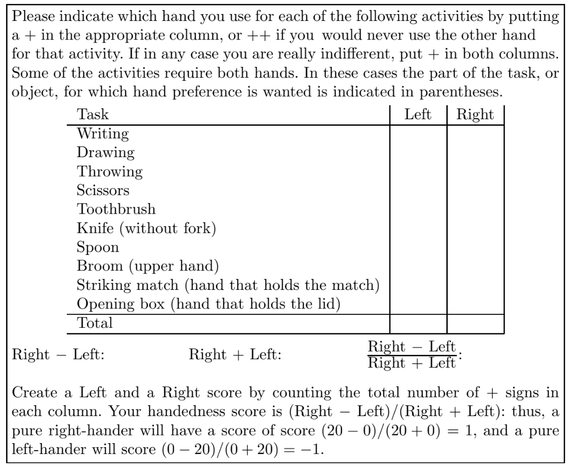
Figure 1.1: Handedness questionnaire (Gelman, 2022)

Question 1.2 Surveys and experiments are often seen as different research methods. Under what conditions, if any, could a survey be considered an experimental study? Discuss.

Question 1.3 Compare quantitative and qualitative variables. Can a variable be both? Why or why not?

Question 1.4 Explain the difference between percent change and percentage points, and why confusing them can lead to misinterpretation.

1.9.2 Test questions

Question 1.5

Which of the following is an example of an observational study?

Testing a new drug in a controlled clinical trial Recording the daily behavior of children in a playground without intervention Randomly assigning participants to two different diets Manipulating fertilizer levels in a plant growth experiment

Question 1.6

Which variable type is discrete quantitative?

Temperature in Celsius Eye color Likert-scale satisfaction ratings Number of students in a classroom

Question 1.7

Which variable is on a ratio scale?

Calendar year Temperature in Celsius Number of cars owned Likert-scale rating

Question 1.8

Which of the following is a nominal variable?

Blood type Height of students Year of birth Temperature in Fahrenheit

Question 1.9

Which of the following is true about interval variables?

Ratios are meaningful They are always qualitative They can only take integer values Differences are meaningful, but zero is arbitrary

Question 1.10

Which of these is a proper use of mode?

Only for numeric variables Only for ordinal variables For all types of variables, including nominal Only for ratio variables

Question 1.11

Which decimal and thousand separators are used in English?

Decimal comma, space for thousands Decimal point, comma for thousands Decimal point, space for thousands Decimal comma, comma for thousands

This division is not always clear-cut. For example, income is technically discrete (values differ by a cent or penny), but it is often modeled as continuous for convenience.↩︎