6.2 Pivoting

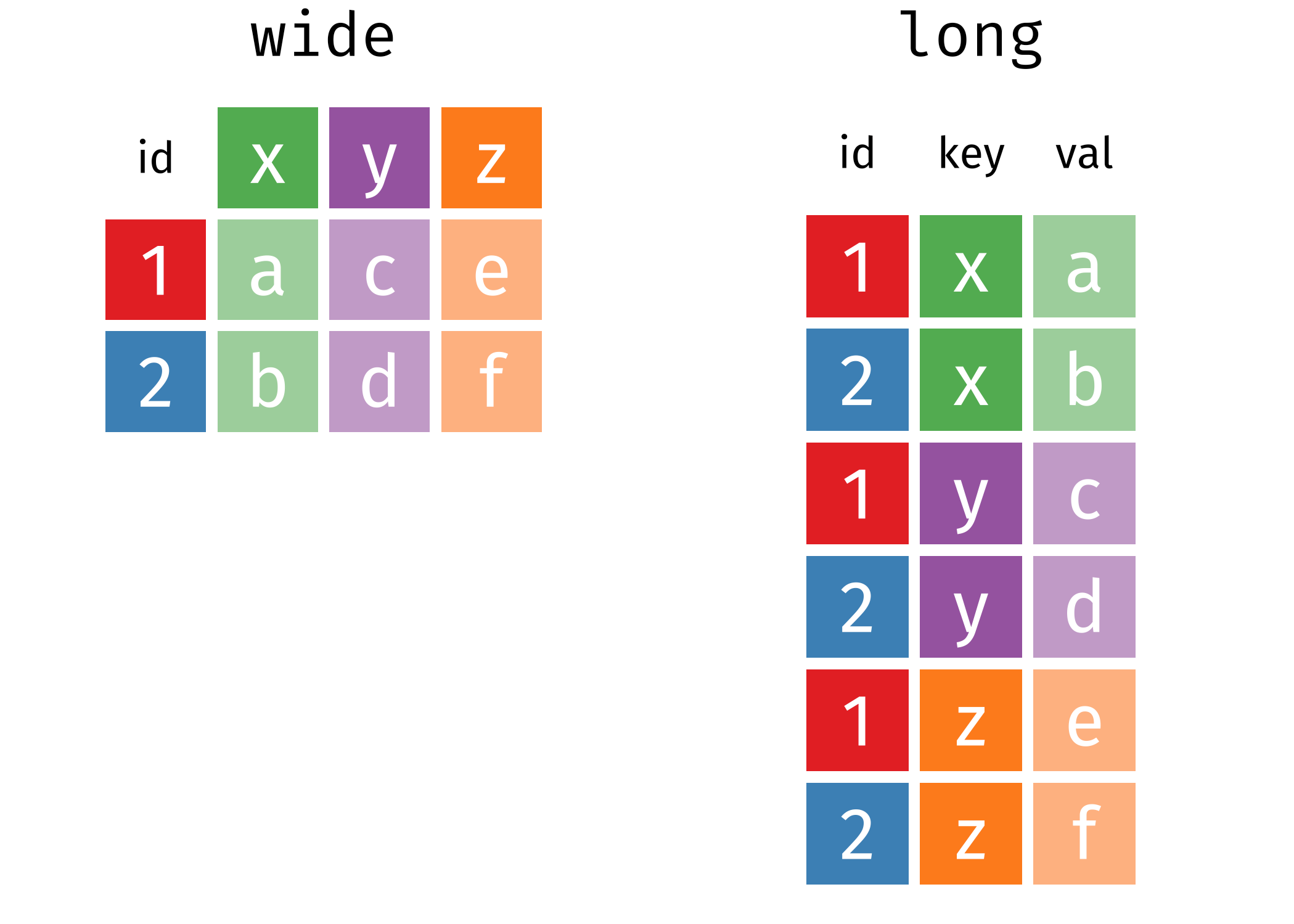
Figure 6.1: Taken from https://www.garrickadenbuie.com/project/tidyexplain/#spread-and-gather

细看两表，不难发现它们实质上相同的数据(相对于第二张表，第一张是以 id 为行字段，key 为列字段，val 为值的数据透视表)。第一种称为宽数据 (wide data,Cartesian data,笛卡尔型数据)，需要看行和列的交叉点来找到对应的值。而第二种形式称为长数据(long data,indexed data，指标型数据)，在长数据（指标型）数据汇总，你需要看指标来找到需要变量的数值（变量x，y，z的值）。。很难简单地说哪一种格式更优，因为两种形式都有可能是整洁的，这取决于值“A”、“B”、“C”、“D”的含义。

数据整理常需要化宽为长，但偶尔也需要化长为宽, tidyr 分别提供了cpivot_longer() 和 pivot_wider() 来实现以上两种形式的转换操作(统称为 pivoting)。在 tidyr 1.0.0 及更早的版本中，gather() 和 spread() 分别承担相同的工作，实际效果与 pivot_ 函数一样，但后者有更易理解的命名和 api。

pivot_longer(data, 
  cols,
  names_to = "name",
  values_to = "value",)

pivot_wider(data, 
  names_from = name,
  values_from = value)

names_to 和 values_to 参数相当于原来 gather() 中的 key 和 value，其中 “键” 列的默认名称变为 “name”
同理, names_from 和 values_from 相当于原来 spread() 中的 key 和 value

6.2.1 pivot_longer()

tidyr::relig_income 是一个典型的宽数据，除第一列以外的所有列表示收入的不同水平，值表示对应的人数：

relig_income 
#> # A tibble: 18 x 11
#>   religion `<$10k` `$10-20k` `$20-30k` `$30-40k` `$40-50k` `$50-75k` `$75-100k`
#>   <chr>      <dbl>     <dbl>     <dbl>     <dbl>     <dbl>     <dbl>      <dbl>
#> 1 Agnostic      27        34        60        81        76       137        122
#> 2 Atheist       12        27        37        52        35        70         73
#> 3 Buddhist      27        21        30        34        33        58         62
#> 4 Catholic     418       617       732       670       638      1116        949
#> 5 Don’t k~      15        14        15        11        10        35         21
#> 6 Evangel~     575       869      1064       982       881      1486        949
#> # ... with 12 more rows, and 3 more variables: `$100-150k` <dbl>,
#> #   `>150k` <dbl>, `Don't know/refused` <dbl>
relig_income %>% pivot_longer(-religion, 
                              names_to = "income", 
                              values_to = "population")
#> pivot_longer: reorganized (<$10k, $10-20k, $20-30k, $30-40k, $40-50k, …) into (income, population) [was 18x11, now 180x3]
#> # A tibble: 180 x 3
#>   religion income  population
#>   <chr>    <chr>        <dbl>
#> 1 Agnostic <$10k           27
#> 2 Agnostic $10-20k         34
#> 3 Agnostic $20-30k         60
#> 4 Agnostic $30-40k         81
#> 5 Agnostic $40-50k         76
#> 6 Agnostic $50-75k        137
#> # ... with 174 more rows

另一个例子：美国劳工市场的月度数据，首先创建一个 messy data：

ec2 <- economics %>% as_tibble() %>%
  transmute(year =  year(date),
            month = month(date),
            rate = unemploy) %>%
  filter(year > 2005) %>% 
  pivot_wider(names_from = "month", values_from = "rate")
#> transmute: dropped 6 variables (date, pce, pop, psavert, uempmed, …)
#>            new variable 'year' with 49 unique values and 0% NA
#>            new variable 'month' with 12 unique values and 0% NA
#>            new variable 'rate' with 550 unique values and 0% NA
#> filter: removed 462 rows (80%), 112 rows remaining
#> pivot_wider: reorganized (month, rate) into (1, 2, 3, 4, 5, …) [was 112x3, now 10x13]
ec2
#> # A tibble: 10 x 13
#>    year   `1`   `2`   `3`   `4`   `5`   `6`   `7`   `8`   `9`  `10`  `11`  `12`
#>   <dbl> <dbl> <dbl> <dbl> <dbl> <dbl> <dbl> <dbl> <dbl> <dbl> <dbl> <dbl> <dbl>
#> 1  2006  7064  7184  7072  7120  6980  7001  7175  7091  6847  6727  6872  6762
#> 2  2007  7116  6927  6731  6850  6766  6979  7149  7067  7170  7237  7240  7645
#> 3  2008  7685  7497  7822  7637  8395  8575  8937  9438  9494 10074 10538 11286
#> 4  2009 12058 12898 13426 13853 14499 14707 14601 14814 15009 15352 15219 15098
#> 5  2010 15046 15113 15202 15325 14849 14474 14512 14648 14579 14516 15081 14348
#> 6  2011 14013 13820 13737 13957 13855 13962 13763 13818 13948 13594 13302 13093
#> # ... with 4 more rows

化宽为长：

ec2 %>% 
  pivot_longer(-year, names_to = "month", values_to = "value")
#> pivot_longer: reorganized (1, 2, 3, 4, 5, …) into (month, value) [was 10x13, now 120x3]
#> # A tibble: 120 x 3
#>    year month value
#>   <dbl> <chr> <dbl>
#> 1  2006 1      7064
#> 2  2006 2      7184
#> 3  2006 3      7072
#> 4  2006 4      7120
#> 5  2006 5      6980
#> 6  2006 6      7001
#> # ... with 114 more rows

以上就是 pviot_longer 的基本用法，下面来处理一些更复杂的情况。

6.2.1.1 Numeric data in column names

pivot_longer() 提供了 names_ptype 和 values_ptypes 调整数据集变长后键列和值列的数据类型。看一下 billboard 数据集：

billboard
#> # A tibble: 317 x 79
#>   artist track date.entered   wk1   wk2   wk3   wk4   wk5   wk6   wk7   wk8
#>   <chr>  <chr> <date>       <dbl> <dbl> <dbl> <dbl> <dbl> <dbl> <dbl> <dbl>
#> 1 2 Pac  Baby~ 2000-02-26      87    82    72    77    87    94    99    NA
#> 2 2Ge+h~ The ~ 2000-09-02      91    87    92    NA    NA    NA    NA    NA
#> 3 3 Doo~ Kryp~ 2000-04-08      81    70    68    67    66    57    54    53
#> 4 3 Doo~ Loser 2000-10-21      76    76    72    69    67    65    55    59
#> 5 504 B~ Wobb~ 2000-04-15      57    34    25    17    17    31    36    49
#> 6 98^0   Give~ 2000-08-19      51    39    34    26    26    19     2     2
#> # ... with 311 more rows, and 68 more variables: wk9 <dbl>, wk10 <dbl>,
#> #   wk11 <dbl>, wk12 <dbl>, wk13 <dbl>, wk14 <dbl>, wk15 <dbl>, wk16 <dbl>,
#> #   wk17 <dbl>, wk18 <dbl>, wk19 <dbl>, wk20 <dbl>, wk21 <dbl>, wk22 <dbl>,
#> #   wk23 <dbl>, wk24 <dbl>, wk25 <dbl>, wk26 <dbl>, wk27 <dbl>, wk28 <dbl>,
#> #   wk29 <dbl>, wk30 <dbl>, wk31 <dbl>, wk32 <dbl>, wk33 <dbl>, wk34 <dbl>,
#> #   wk35 <dbl>, wk36 <dbl>, wk37 <dbl>, wk38 <dbl>, wk39 <dbl>, wk40 <dbl>,
#> #   wk41 <dbl>, wk42 <dbl>, wk43 <dbl>, wk44 <dbl>, wk45 <dbl>, wk46 <dbl>,
#> #   wk47 <dbl>, wk48 <dbl>, wk49 <dbl>, wk50 <dbl>, wk51 <dbl>, wk52 <dbl>,
#> #   wk53 <dbl>, wk54 <dbl>, wk55 <dbl>, wk56 <dbl>, wk57 <dbl>, wk58 <dbl>,
#> #   wk59 <dbl>, wk60 <dbl>, wk61 <dbl>, wk62 <dbl>, wk63 <dbl>, wk64 <dbl>,
#> #   wk65 <dbl>, wk66 <lgl>, wk67 <lgl>, wk68 <lgl>, wk69 <lgl>, wk70 <lgl>,
#> #   wk71 <lgl>, wk72 <lgl>, wk73 <lgl>, wk74 <lgl>, wk75 <lgl>, wk76 <lgl>

显然，我们希望将所有以 "wk"开头的列聚合以得到整洁数据，键列和值列分别命名为 “week” 和 “rank”。另外要考虑的一点是，我们很可能之后想计算歌曲保持在榜单上的周数，故需要将 “week” 列转换为数值类型：

billboard_tidy <- billboard %>% 
  pivot_longer(cols = starts_with("wk"),
               names_to = "week",
               values_to = "rank",
               names_prefix = "wk",
               names_ptypes = list(week = integer()),
               values_drop_na = T)
#> pivot_longer: reorganized (wk1, wk2, wk3, wk4, wk5, …) into (week, rank) [was 317x79, now 5307x5]

billboard_tidy
#> # A tibble: 5,307 x 5
#>   artist track                   date.entered  week  rank
#>   <chr>  <chr>                   <date>       <int> <dbl>
#> 1 2 Pac  Baby Don't Cry (Keep... 2000-02-26       1    87
#> 2 2 Pac  Baby Don't Cry (Keep... 2000-02-26       2    82
#> 3 2 Pac  Baby Don't Cry (Keep... 2000-02-26       3    72
#> 4 2 Pac  Baby Don't Cry (Keep... 2000-02-26       4    77
#> 5 2 Pac  Baby Don't Cry (Keep... 2000-02-26       5    87
#> 6 2 Pac  Baby Don't Cry (Keep... 2000-02-26       6    94
#> # ... with 5,301 more rows

names_prefix 去除前缀 “wk”(否则无法从字符串转换为数值)，names_ptype 以列表的形式转换键列的数据类型。同理, values_ptype 可以转换值列的数据类型。

## 计算保持周数
billboard_tidy %>% 
  group_by(track) %>% 
  summarise(stay = max(week) - min(week) + 1) %>% 
  arrange(desc(stay))
#> group_by: one grouping variable (track)
#> summarise: now 316 rows and 2 columns, ungrouped
#> # A tibble: 316 x 2
#>   track                stay
#>   <chr>               <dbl>
#> 1 Higher                 65
#> 2 Amazed                 64
#> 3 Breathe                53
#> 4 Kryptonite             53
#> 5 With Arms Wide Open    47
#> 6 I Wanna Know           44
#> # ... with 310 more rows

6.2.1.2 Many variables in column names

在 tidyr 1.0.0 之前，当进行一定处理后发现多个变量被糅合到一列中时，可能会考虑使用 separate() 或者 extract():

who
#> # A tibble: 7,240 x 60
#>   country iso2  iso3   year new_sp_m014 new_sp_m1524 new_sp_m2534 new_sp_m3544
#>   <chr>   <chr> <chr> <int>       <int>        <int>        <int>        <int>
#> 1 Afghan~ AF    AFG    1980          NA           NA           NA           NA
#> 2 Afghan~ AF    AFG    1981          NA           NA           NA           NA
#> 3 Afghan~ AF    AFG    1982          NA           NA           NA           NA
#> 4 Afghan~ AF    AFG    1983          NA           NA           NA           NA
#> 5 Afghan~ AF    AFG    1984          NA           NA           NA           NA
#> 6 Afghan~ AF    AFG    1985          NA           NA           NA           NA
#> # ... with 7,234 more rows, and 52 more variables: new_sp_m4554 <int>,
#> #   new_sp_m5564 <int>, new_sp_m65 <int>, new_sp_f014 <int>,
#> #   new_sp_f1524 <int>, new_sp_f2534 <int>, new_sp_f3544 <int>,
#> #   new_sp_f4554 <int>, new_sp_f5564 <int>, new_sp_f65 <int>,
#> #   new_sn_m014 <int>, new_sn_m1524 <int>, new_sn_m2534 <int>,
#> #   new_sn_m3544 <int>, new_sn_m4554 <int>, new_sn_m5564 <int>,
#> #   new_sn_m65 <int>, new_sn_f014 <int>, new_sn_f1524 <int>,
#> #   new_sn_f2534 <int>, new_sn_f3544 <int>, new_sn_f4554 <int>,
#> #   new_sn_f5564 <int>, new_sn_f65 <int>, new_ep_m014 <int>,
#> #   new_ep_m1524 <int>, new_ep_m2534 <int>, new_ep_m3544 <int>,
#> #   new_ep_m4554 <int>, new_ep_m5564 <int>, new_ep_m65 <int>,
#> #   new_ep_f014 <int>, new_ep_f1524 <int>, new_ep_f2534 <int>,
#> #   new_ep_f3544 <int>, new_ep_f4554 <int>, new_ep_f5564 <int>,
#> #   new_ep_f65 <int>, newrel_m014 <int>, newrel_m1524 <int>,
#> #   newrel_m2534 <int>, newrel_m3544 <int>, newrel_m4554 <int>,
#> #   newrel_m5564 <int>, newrel_m65 <int>, newrel_f014 <int>,
#> #   newrel_f1524 <int>, newrel_f2534 <int>, newrel_f3544 <int>,
#> #   newrel_f4554 <int>, newrel_f5564 <int>, newrel_f65 <int>
## 原书 tidyr 一章中使用的方法
who %>% 
  gather(starts_with("new"), 
         key = key, 
         value = value,
         na.rm = T) %>% 
  extract(key,
          into = c("diagnosis", "gender", "age"),
          regex = "new_?(.*)_(.)(.*)")
#> gather: reorganized (new_sp_m014, new_sp_m1524, new_sp_m2534, new_sp_m3544, new_sp_m4554, …) into (key, value) [was 7240x60, now 76046x6]
#> # A tibble: 76,046 x 8
#>   country     iso2  iso3   year diagnosis gender age   value
#>   <chr>       <chr> <chr> <int> <chr>     <chr>  <chr> <int>
#> 1 Afghanistan AF    AFG    1997 sp        m      014       0
#> 2 Afghanistan AF    AFG    1998 sp        m      014      30
#> 3 Afghanistan AF    AFG    1999 sp        m      014       8
#> 4 Afghanistan AF    AFG    2000 sp        m      014      52
#> 5 Afghanistan AF    AFG    2001 sp        m      014     129
#> 6 Afghanistan AF    AFG    2002 sp        m      014      90
#> # ... with 76,040 more rows

现在，pivot_longer() 现在可以在化宽为长的下一步直接完成拆分任务，可以直接在 names_to 中传入一个向量表示分裂后的各个键列，并在 names_sep(分隔符) 或者 names_pattern 中(正则表达式)指定分裂的模式：

who %>% 
  pivot_longer(starts_with("new"),
               names_to = c("diagonosis", "gender", "age"),
               names_pattern = "new_?(.*)_(.)(.*)",
               values_to = "count",
               values_drop_na = T)
#> pivot_longer: reorganized (new_sp_m014, new_sp_m1524, new_sp_m2534, new_sp_m3544, new_sp_m4554, …) into (diagonosis, gender, age, count) [was 7240x60, now 76046x8]
#> # A tibble: 76,046 x 8
#>   country     iso2  iso3   year diagonosis gender age   count
#>   <chr>       <chr> <chr> <int> <chr>      <chr>  <chr> <int>
#> 1 Afghanistan AF    AFG    1997 sp         m      014       0
#> 2 Afghanistan AF    AFG    1997 sp         m      1524     10
#> 3 Afghanistan AF    AFG    1997 sp         m      2534      6
#> 4 Afghanistan AF    AFG    1997 sp         m      3544      3
#> 5 Afghanistan AF    AFG    1997 sp         m      4554      5
#> 6 Afghanistan AF    AFG    1997 sp         m      5564      2
#> # ... with 76,040 more rows

更进一步，顺便设定好整理后 gender 和 age 的类型：

who %>% 
  pivot_longer(cols = starts_with("new"),
               names_to = c("diagonosis", "gender", "age"),
               names_pattern = "new_?(.*)_(.)(.*)",
               names_ptypes = list(
                 gender = factor(levels = c("f", "m")),
                 age = factor(
                        levels = c("014", "1524", "2534", "3544", "4554", "5564", "65"), 
                        ordered = TRUE)
               ),
               values_to = "count",
               values_drop_na = T)
#> pivot_longer: reorganized (new_sp_m014, new_sp_m1524, new_sp_m2534, new_sp_m3544, new_sp_m4554, …) into (diagonosis, gender, age, count) [was 7240x60, now 76046x8]
#> # A tibble: 76,046 x 8
#>   country     iso2  iso3   year diagonosis gender age   count
#>   <chr>       <chr> <chr> <int> <chr>      <fct>  <ord> <int>
#> 1 Afghanistan AF    AFG    1997 sp         m      014       0
#> 2 Afghanistan AF    AFG    1997 sp         m      1524     10
#> 3 Afghanistan AF    AFG    1997 sp         m      2534      6
#> 4 Afghanistan AF    AFG    1997 sp         m      3544      3
#> 5 Afghanistan AF    AFG    1997 sp         m      4554      5
#> 6 Afghanistan AF    AFG    1997 sp         m      5564      2
#> # ... with 76,040 more rows

6.2.1.3 Multiple observations per row

(多个值列)

So far, we have been working with data frames that have one observation per row, but many important pivotting problems involve multiple observations per row. You can usually recognise this case because name of the column that you want to appear in the output is part of the column name in the input. In this section, you’ll learn how to pivot this sort of data.

family <- tribble(
  ~family,  ~dob_child1,  ~dob_child2, ~gender_child1, ~gender_child2,
       1L, "1998-11-26", "2000-01-29",             1L,             2L,
       2L, "1996-06-22",           NA,             2L,             NA,
       3L, "2002-07-11", "2004-04-05",             2L,             2L,
       4L, "2004-10-10", "2009-08-27",             1L,             1L,
       5L, "2000-12-05", "2005-02-28",             2L,             1L,
)
family <- family %>% mutate_at(vars(starts_with("dob")), ymd)
#> mutate_at: converted 'dob_child1' from character to Date (0 new NA)
#>            converted 'dob_child2' from character to Date (0 new NA)
family
#> # A tibble: 5 x 5
#>   family dob_child1 dob_child2 gender_child1 gender_child2
#>    <int> <date>     <date>             <int>         <int>
#> 1      1 1998-11-26 2000-01-29             1             2
#> 2      2 1996-06-22 NA                     2            NA
#> 3      3 2002-07-11 2004-04-05             2             2
#> 4      4 2004-10-10 2009-08-27             1             1
#> 5      5 2000-12-05 2005-02-28             2             1

理想中的数据格式(两个值列)

family	child	dob	gender
1	1	1998-11-26	1
1	2	2000-01-29	2
2	1	1996-06-22	2
3	1	2002-07-11	2
3	2	2004-04-05	2
4	1	2004-10-10	1
4	2	2009-08-27	1
5	1	2000-12-05	2
5	2	2005-02-28	1

Note that we have two pieces of information (or values) for each child: their gender and their dob (date of birth). These need to go into separate columns in the result. Again we supply multiple variables to names_to, using names_sep to split up each variable name. Note the special name .value: this tells pivot_longer() that that part of the column name specifies the “value” being measured (which will become a variable in the output)

.value 在这里指代 dob 和 gender 两个值列

family %>% 
  pivot_longer(
    -family, 
    names_to = c(".value", "child"),   ## child 为每个 family 中的标识变量
    names_sep = "_", 
    values_drop_na = TRUE
  )
#> pivot_longer: reorganized (dob_child1, dob_child2, gender_child1, gender_child2) into (child, dob, gender) [was 5x5, now 9x4]
#> # A tibble: 9 x 4
#>   family child  dob        gender
#>    <int> <chr>  <date>      <int>
#> 1      1 child1 1998-11-26      1
#> 2      1 child2 2000-01-29      2
#> 3      2 child1 1996-06-22      2
#> 4      3 child1 2002-07-11      2
#> 5      3 child2 2004-04-05      2
#> 6      4 child1 2004-10-10      1
#> # ... with 3 more rows

在这里，dob_child1、dob_child2、gender_child1、gender_child2四个列名的后半部分被当做键列的值。例如，可以认为对于 family == 1的观测，首先生成了如下的结构：

family	child	dob	dob	gender	gender
1	child1	1998-11-16	2000-01-29	1	2
2	child2

而后名称相同的值列合并：

family	child	dob	gender
1	child1	1998-11-26	1
1	child2	2000-01-29	2

另一个例子：

anscombe 
#>    x1 x2 x3 x4    y1   y2    y3    y4
#> 1  10 10 10  8  8.04 9.14  7.46  6.58
#> 2   8  8  8  8  6.95 8.14  6.77  5.76
#> 3  13 13 13  8  7.58 8.74 12.74  7.71
#> 4   9  9  9  8  8.81 8.77  7.11  8.84
#> 5  11 11 11  8  8.33 9.26  7.81  8.47
#> 6  14 14 14  8  9.96 8.10  8.84  7.04
#> 7   6  6  6  8  7.24 6.13  6.08  5.25
#> 8   4  4  4 19  4.26 3.10  5.39 12.50
#> 9  12 12 12  8 10.84 9.13  8.15  5.56
#> 10  7  7  7  8  4.82 7.26  6.42  7.91
#> 11  5  5  5  8  5.68 4.74  5.73  6.89
anscombe %>% 
  pivot_longer(everything(),
               names_to = c(".value", "set"),
               names_pattern = "([xy])([1234])")
#> pivot_longer: reorganized (x1, x2, x3, x4, y1, …) into (set, x, y) [was 11x8, now 44x3]
#> # A tibble: 44 x 3
#>   set       x     y
#>   <chr> <dbl> <dbl>
#> 1 1        10  8.04
#> 2 2        10  9.14
#> 3 3        10  7.46
#> 4 4         8  6.58
#> 5 1         8  6.95
#> 6 2         8  8.14
#> # ... with 38 more rows

叕一个例子：

pnl <- tibble(
  x = 1:4,
  a = c(1, 1,0, 0),
  b = c(0, 1, 1, 1),
  y1 = rnorm(4),
  y2 = rnorm(4),
  z1 = rep(3, 4),
  z2 = rep(-2, 4),
)
pnl
#> # A tibble: 4 x 7
#>       x     a     b      y1     y2    z1    z2
#>   <int> <dbl> <dbl>   <dbl>  <dbl> <dbl> <dbl>
#> 1     1     1     0  0.788  -1.59      3    -2
#> 2     2     1     1 -0.422   0.597     3    -2
#> 3     3     0     1  0.0569  1.22      3    -2
#> 4     4     0     1  0.711  -0.312     3    -2

pnl %>% 
  pivot_longer(-(x:b),
               names_to = c(".value", "time"),
               names_pattern = "([yz])([12])")
#> pivot_longer: reorganized (y1, y2, z1, z2) into (time, y, z) [was 4x7, now 8x6]
#> # A tibble: 8 x 6
#>       x     a     b time        y     z
#>   <int> <dbl> <dbl> <chr>   <dbl> <dbl>
#> 1     1     1     0 1      0.788      3
#> 2     1     1     0 2     -1.59      -2
#> 3     2     1     1 1     -0.422      3
#> 4     2     1     1 2      0.597     -2
#> 5     3     0     1 1      0.0569     3
#> 6     3     0     1 2      1.22      -2
#> # ... with 2 more rows

6.2.1.4 Duplicated column names

如果某个数据框中各列有重复的名字，用 gather() 聚合这些变量所在的列时会返回一条错误：

Error: Can't bind data because some arguments have the same name

这是因为被聚合的列名被当做 key 列的值，又因这些值是重复的，故不能唯一标识一条记录。pivot_longer() 针对这一点做了优化，尝试聚合这些列时，会自动生成一个标识列：

#  To create a tibble with duplicated names
# you have to explicitly opt out of the name repair 
# that usually prevents you from creating such a dataset:
(df <- tibble(x = 1:3, y = 4:6, y = 5:7, y = 7:9, .name_repair = "minimal")) 
#> # A tibble: 3 x 4
#>       x     y     y     y
#>   <int> <int> <int> <int>
#> 1     1     4     5     7
#> 2     2     5     6     8
#> 3     3     6     7     9

df %>% 
  pivot_longer(-x, names_to = "y")
#> pivot_longer: reorganized () into (.copy, value) [was 3x4, now 9x4]
#> # A tibble: 9 x 4
#>       x y     .copy value
#>   <int> <chr> <int> <int>
#> 1     1 y         1     4
#> 2     1 y         2     5
#> 3     1 y         3     7
#> 4     2 y         1     5
#> 5     2 y         2     6
#> 6     2 y         3     8
#> # ... with 3 more rows

6.2.2 pivot_wider()

pivot_wider() 是 pivot_longer() 的逆操作，虽然在获得 tidy data 上，前者没有后者常用，但它经常被用来创建一些 summary table。

fish_encounters 数据记录了一些沿河观测站对一批鱼群的观测情况(seen 为发现次数)：

fish_encounters
#> # A tibble: 114 x 3
#>   fish  station  seen
#>   <fct> <fct>   <int>
#> 1 4842  Release     1
#> 2 4842  I80_1       1
#> 3 4842  Lisbon      1
#> 4 4842  Rstr        1
#> 5 4842  Base_TD     1
#> 6 4842  BCE         1
#> # ... with 108 more rows

很多后续分析工具需要每个观测站的观测情况单独成一列，使用 pivot_wider():

# 数据中已有的列不需要引号便可引用
fish_encounters %>% 
  pivot_wider(names_from = station, values_from = seen)
#> pivot_wider: reorganized (station, seen) into (Release, I80_1, Lisbon, Rstr, Base_TD, …) [was 114x3, now 19x12]
#> # A tibble: 19 x 12
#>   fish  Release I80_1 Lisbon  Rstr Base_TD   BCE   BCW  BCE2  BCW2   MAE   MAW
#>   <fct>   <int> <int>  <int> <int>   <int> <int> <int> <int> <int> <int> <int>
#> 1 4842        1     1      1     1       1     1     1     1     1     1     1
#> 2 4843        1     1      1     1       1     1     1     1     1     1     1
#> 3 4844        1     1      1     1       1     1     1     1     1     1     1
#> 4 4845        1     1      1     1       1    NA    NA    NA    NA    NA    NA
#> 5 4847        1     1      1    NA      NA    NA    NA    NA    NA    NA    NA
#> 6 4848        1     1      1     1      NA    NA    NA    NA    NA    NA    NA
#> # ... with 13 more rows

关于 pivot_wider()，很重要的一点是它会暴露出数据中的隐式缺失值(implicit missing value)。这些没有出现在原数据中的 NA 值不是源自于记录错误或者遗失，只是没有对应的观测而已（观测站只能记录发生了的观测）。参数 values_fill 可以以一个列表填充 pivot_wider() 结果中的 NA， 当然如何处理这些隐式缺失值要按具体情境而定，在鱼群的例子里，用 0 填充是合适的：

fish_encounters %>% 
  pivot_wider(names_from = station, values_from = seen,
              values_fill = list(seen = 0))
#> pivot_wider: reorganized (station, seen) into (Release, I80_1, Lisbon, Rstr, Base_TD, …) [was 114x3, now 19x12]
#> # A tibble: 19 x 12
#>   fish  Release I80_1 Lisbon  Rstr Base_TD   BCE   BCW  BCE2  BCW2   MAE   MAW
#>   <fct>   <int> <int>  <int> <int>   <int> <int> <int> <int> <int> <int> <int>
#> 1 4842        1     1      1     1       1     1     1     1     1     1     1
#> 2 4843        1     1      1     1       1     1     1     1     1     1     1
#> 3 4844        1     1      1     1       1     1     1     1     1     1     1
#> 4 4845        1     1      1     1       1     0     0     0     0     0     0
#> 5 4847        1     1      1     0       0     0     0     0     0     0     0
#> 6 4848        1     1      1     1       0     0     0     0     0     0     0
#> # ... with 13 more rows

fish_encoutners 的贡献者 Myfanwy Johnston 在个人网站上有一篇相关的文章

6.2.2.1 Aggregation

pivot_wider() 可以用来执行一些简单的聚合操作。warpbreaks 是一个关于经纱强度的控制试验，每个处理 (wool, tension) 上进行了 9 次试验：

(warpbreaks <- warpbreaks %>% as_tibble() %>% select(wool, tension, breaks))
#> select: columns reordered (wool, tension, breaks)
#> # A tibble: 54 x 3
#>   wool  tension breaks
#>   <fct> <fct>    <dbl>
#> 1 A     L           26
#> 2 A     L           30
#> 3 A     L           54
#> 4 A     L           25
#> 5 A     L           70
#> 6 A     L           52
#> # ... with 48 more rows
warpbreaks %>% count(wool, tension)
#> count: now 6 rows and 3 columns, ungrouped
#> # A tibble: 6 x 3
#>   wool  tension     n
#>   <fct> <fct>   <int>
#> 1 A     L           9
#> 2 A     M           9
#> 3 A     H           9
#> 4 B     L           9
#> 5 B     M           9
#> 6 B     H           9

现在想知道每个处理下的平均断头次数，只需展开 wool 或 tension 中的任意一个：

warpbreaks %>% 
  pivot_wider(names_from = wool, values_from = breaks)
#> Warning: Values in `breaks` are not uniquely identified; output will contain list-cols.
#> * Use `values_fn = list(breaks = list)` to suppress this warning.
#> * Use `values_fn = list(breaks = length)` to identify where the duplicates arise
#> * Use `values_fn = list(breaks = summary_fun)` to summarise duplicates
#> pivot_wider: reorganized (wool, breaks) into (A, B) [was 54x3, now 3x3]
#> # A tibble: 3 x 3
#>   tension A         B        
#>   <fct>   <list>    <list>   
#> 1 L       <dbl [9]> <dbl [9]>
#> 2 M       <dbl [9]> <dbl [9]>
#> 3 H       <dbl [9]> <dbl [9]>

由于 (wool, tension) 不能唯一确认一个观测，多个观测被压缩至一个列表中，values_fn(breaks = mean) 求得平均值：

warpbreaks %>% 
  pivot_wider(names_from = wool, values_from = breaks,
              values_fn = list(breaks = mean))
#> pivot_wider: reorganized (wool, breaks) into (A, B) [was 54x3, now 3x3]
#> # A tibble: 3 x 3
#>   tension     A     B
#>   <fct>   <dbl> <dbl>
#> 1 L        44.6  28.2
#> 2 M        24    28.8
#> 3 H        24.6  18.8

For more complex summary operations, I recommend summarising before reshaping, but for simple cases it’s often convenient to summarise within pivot_wider()

6.2.2.2 Generate column name from multiple variables

现有一个数据集存储了关于产品、生产国家、生产年份和产量的水平组合：

production <- expand_grid(
    product = c("A", "B"), 
    country = c("AI", "EI"), 
    year = 2000:2014
  ) %>%
  filter((product == "A" & country == "AI") | product == "B") %>% 
  mutate(production = rnorm(nrow(.)))
#> filter: removed 15 rows (25%), 45 rows remaining
#> mutate: new variable 'production' with 45 unique values and 0% NA

production
#> # A tibble: 45 x 4
#>   product country  year production
#>   <chr>   <chr>   <int>      <dbl>
#> 1 A       AI       2000     -0.209
#> 2 A       AI       2001     -0.369
#> 3 A       AI       2002      0.330
#> 4 A       AI       2003      1.88 
#> 5 A       AI       2004     -0.482
#> 6 A       AI       2005      1.74 
#> # ... with 39 more rows

假设现在希望对于每个 product 和 country 的组合均创建一列，关键是在 names_from 中传入一个向量：

production %>% 
  pivot_wider(names_from = c(product, country), values_from = production)
#> pivot_wider: reorganized (product, country, production) into (A_AI, B_AI, B_EI) [was 45x4, now 15x4]
#> # A tibble: 15 x 4
#>    year   A_AI   B_AI    B_EI
#>   <int>  <dbl>  <dbl>   <dbl>
#> 1  2000 -0.209  1.02  -1.14  
#> 2  2001 -0.369  0.598  0.143 
#> 3  2002  0.330  1.38  -0.0472
#> 4  2003  1.88  -1.06  -1.26  
#> 5  2004 -0.482  0.197  3.39  
#> 6  2005  1.74   1.37   0.120 
#> # ... with 9 more rows

names_sep 可以指定除了 _ 以外的分隔符。names_prefix 为展开后的各列添加前缀(as opposed to removing in pivot_longer())

6.2.2.3 Multiple value columns

The us_rent_income dataset contains information about median income and rent for each state in the US for 2017 (from the American Community Survey, retrieved with the tidycensus package).

us_rent_income
#> # A tibble: 104 x 5
#>   GEOID NAME    variable estimate   moe
#>   <chr> <chr>   <chr>       <dbl> <dbl>
#> 1 01    Alabama income      24476   136
#> 2 01    Alabama rent          747     3
#> 3 02    Alaska  income      32940   508
#> 4 02    Alaska  rent         1200    13
#> 5 04    Arizona income      27517   148
#> 6 04    Arizona rent          972     4
#> # ... with 98 more rows

Here both estimate and moe are values columns, so we can supply them to values_from:

us_rent_income %>% pivot_wider(names_from = variable, values_from = c(estimate, moe))
#> pivot_wider: reorganized (variable, estimate, moe) into (estimate_income, estimate_rent, moe_income, moe_rent) [was 104x5, now 52x6]
#> # A tibble: 52 x 6
#>   GEOID NAME       estimate_income estimate_rent moe_income moe_rent
#>   <chr> <chr>                <dbl>         <dbl>      <dbl>    <dbl>
#> 1 01    Alabama              24476           747        136        3
#> 2 02    Alaska               32940          1200        508       13
#> 3 04    Arizona              27517           972        148        4
#> 4 05    Arkansas             23789           709        165        5
#> 5 06    California           29454          1358        109        3
#> 6 08    Colorado             32401          1125        109        5
#> # ... with 46 more rows

Note that the name of the variable is automatically appended to the output columns.

6.2.2.4 When there is no identifying variable

A final challenge is inspired by Jiena Gu. Imagine you have a contact list that you’ve copied and pasted from a website:

contacts <- tribble(
  ~field, ~value,
  "name", "Jiena McLellan",
  "company", "Toyota", 
  "name", "John Smith", 
  "company", "google", 
  "email", "john@google.com",
  "name", "Huxley Ratcliffe"
)
contacts
#> # A tibble: 6 x 2
#>   field   value           
#>   <chr>   <chr>           
#> 1 name    Jiena McLellan  
#> 2 company Toyota          
#> 3 name    John Smith      
#> 4 company google          
#> 5 email   john@google.com 
#> 6 name    Huxley Ratcliffe

This is challenging because there’s no variable that identifies which observations belong together.

直接化宽时，出现列表列（没有第三个标识变量）

contacts %>% pivot_wider(names_from = field, values_from = value)
#> pivot_wider: reorganized (field, value) into (name, company, email) [was 6x2, now 1x3]
#> # A tibble: 1 x 3
#>   name      company   email    
#>   <list>    <list>    <list>   
#> 1 <chr [3]> <chr [2]> <chr [1]>

We can fix this by noting that every contact starts with a name, so we can create a unique id by counting every time we see “name” as the field:

(contacts <- contacts %>% 
  mutate(
    person_id = cumsum(field == "name")
  ))
#> mutate: new variable 'person_id' with 3 unique values and 0% NA
#> # A tibble: 6 x 3
#>   field   value            person_id
#>   <chr>   <chr>                <int>
#> 1 name    Jiena McLellan           1
#> 2 company Toyota                   1
#> 3 name    John Smith               2
#> 4 company google                   2
#> 5 email   john@google.com          2
#> 6 name    Huxley Ratcliffe         3

contacts %>% 
  pivot_wider(names_from = field, values_from = value)
#> pivot_wider: reorganized (field, value) into (name, company, email) [was 6x3, now 3x4]
#> # A tibble: 3 x 4
#>   person_id name             company email          
#>       <int> <chr>            <chr>   <chr>          
#> 1         1 Jiena McLellan   Toyota  <NA>           
#> 2         2 John Smith       google  john@google.com
#> 3         3 Huxley Ratcliffe <NA>    <NA>

6.2.3 Combining pivot_longer() and pivot_wider()

Some problems can’t be solved by pivotting in a single direction. The examples in this section show how you might combine pivot_longer() and pivot_wider() to solve more complex problems.

6.2.3.1 world bank data

world_bank_pop contains data from the World Bank about population per country from 2000 to 2018.

world_bank_pop
#> # A tibble: 1,056 x 20
#>   country indicator `2000` `2001` `2002` `2003`  `2004`  `2005`   `2006`
#>   <chr>   <chr>      <dbl>  <dbl>  <dbl>  <dbl>   <dbl>   <dbl>    <dbl>
#> 1 ABW     SP.URB.T~ 4.24e4 4.30e4 4.37e4 4.42e4 4.47e+4 4.49e+4  4.49e+4
#> 2 ABW     SP.URB.G~ 1.18e0 1.41e0 1.43e0 1.31e0 9.51e-1 4.91e-1 -1.78e-2
#> 3 ABW     SP.POP.T~ 9.09e4 9.29e4 9.50e4 9.70e4 9.87e+4 1.00e+5  1.01e+5
#> 4 ABW     SP.POP.G~ 2.06e0 2.23e0 2.23e0 2.11e0 1.76e+0 1.30e+0  7.98e-1
#> 5 AFG     SP.URB.T~ 4.44e6 4.65e6 4.89e6 5.16e6 5.43e+6 5.69e+6  5.93e+6
#> 6 AFG     SP.URB.G~ 3.91e0 4.66e0 5.13e0 5.23e0 5.12e+0 4.77e+0  4.12e+0
#> # ... with 1,050 more rows, and 11 more variables: `2007` <dbl>, `2008` <dbl>,
#> #   `2009` <dbl>, `2010` <dbl>, `2011` <dbl>, `2012` <dbl>, `2013` <dbl>,
#> #   `2014` <dbl>, `2015` <dbl>, `2016` <dbl>, `2017` <dbl>

It’s not obvious exactly what steps are needed yet, but I’ll start with the most obvious problem: year is spread across multiple columns.

pop2 <- world_bank_pop %>% 
  pivot_longer(`2000`:`2017`, names_to = "year", values_to = "value")
#> pivot_longer: reorganized (2000, 2001, 2002, 2003, 2004, …) into (year, value) [was 1056x20, now 19008x4]
pop2
#> # A tibble: 19,008 x 4
#>   country indicator   year  value
#>   <chr>   <chr>       <chr> <dbl>
#> 1 ABW     SP.URB.TOTL 2000  42444
#> 2 ABW     SP.URB.TOTL 2001  43048
#> 3 ABW     SP.URB.TOTL 2002  43670
#> 4 ABW     SP.URB.TOTL 2003  44246
#> 5 ABW     SP.URB.TOTL 2004  44669
#> 6 ABW     SP.URB.TOTL 2005  44889
#> # ... with 19,002 more rows

Next we need to consider the indicator variable:

world_bank_pop %>% count(indicator)
#> count: now 4 rows and 2 columns, ungrouped
#> # A tibble: 4 x 2
#>   indicator       n
#>   <chr>       <int>
#> 1 SP.POP.GROW   264
#> 2 SP.POP.TOTL   264
#> 3 SP.URB.GROW   264
#> 4 SP.URB.TOTL   264

Here SP.POP.GROW is population growth, SP.POP.TOTL is total population, and SP.URB.* are the same but only for urban areas. Let’s split this up into two variables: area (total or urban) and the actual variable (population or growth):

# Use NA to omit the variable in the output.
pop3 <- pop2 %>% 
  separate(indicator, c(NA, "area", "variable"), sep = "\\.")  # sep takes a regex
pop3
#> # A tibble: 19,008 x 5
#>   country area  variable year  value
#>   <chr>   <chr> <chr>    <chr> <dbl>
#> 1 ABW     URB   TOTL     2000  42444
#> 2 ABW     URB   TOTL     2001  43048
#> 3 ABW     URB   TOTL     2002  43670
#> 4 ABW     URB   TOTL     2003  44246
#> 5 ABW     URB   TOTL     2004  44669
#> 6 ABW     URB   TOTL     2005  44889
#> # ... with 19,002 more rows

Now we can complete the tidying by pivoting variable and value to make TOTL and GROW columns:

pop3 %>% 
  pivot_wider(names_from = variable, values_from = value)
#> pivot_wider: reorganized (variable, value) into (TOTL, GROW) [was 19008x5, now 9504x5]
#> # A tibble: 9,504 x 5
#>   country area  year   TOTL  GROW
#>   <chr>   <chr> <chr> <dbl> <dbl>
#> 1 ABW     URB   2000  42444 1.18 
#> 2 ABW     URB   2001  43048 1.41 
#> 3 ABW     URB   2002  43670 1.43 
#> 4 ABW     URB   2003  44246 1.31 
#> 5 ABW     URB   2004  44669 0.951
#> 6 ABW     URB   2005  44889 0.491
#> # ... with 9,498 more rows

6.2.3.2 mutli choice data

Based on a suggestion by Maxime Wack, https://github.com/tidyverse/tidyr/issues/384), the final example shows how to deal with a common way of recording multiple choice data. Often you will get such data as follows:

(multi <- tribble(
  ~id, ~choice1, ~choice2, ~choice3,
  1, "A", "B", "C",
  2, "C", "B",  NA,
  3, "D",  NA,  NA,
  4, "B", "D",  NA
))
#> # A tibble: 4 x 4
#>      id choice1 choice2 choice3
#>   <dbl> <chr>   <chr>   <chr>  
#> 1     1 A       B       C      
#> 2     2 C       B       <NA>   
#> 3     3 D       <NA>    <NA>   
#> 4     4 B       D       <NA>

But the actual order isn’t important, and you’d prefer to have the individual questions in the columns. You can achieve the desired transformation in two steps. First, you make the data longer, eliminating the explcit NAs, and adding a column to indicate that this choice was chosen:

multi2 <- multi %>% 
  pivot_longer(-id, values_drop_na = TRUE) %>% 
  mutate(checked = TRUE)
#> pivot_longer: reorganized (choice1, choice2, choice3) into (name, value) [was 4x4, now 8x3]
#> mutate: new variable 'checked' with one unique value and 0% NA
multi2
#> # A tibble: 8 x 4
#>      id name    value checked
#>   <dbl> <chr>   <chr> <lgl>  
#> 1     1 choice1 A     TRUE   
#> 2     1 choice2 B     TRUE   
#> 3     1 choice3 C     TRUE   
#> 4     2 choice1 C     TRUE   
#> 5     2 choice2 B     TRUE   
#> 6     3 choice1 D     TRUE   
#> # ... with 2 more rows

Then you make the data wider, filling in the missing observations with FALSE; note the use of id_cols = id here, this eliminated the name column and combines mutilples rows per person into one row, since we don’t need name in identifying an observation:

multi2 %>% 
  pivot_wider(id_cols = id,
              names_from = value, values_from = checked, 
              values_fill = list(checked = FALSE))
#> pivot_wider: reorganized (name, value, checked) into (A, B, C, D) [was 8x4, now 4x5]
#> # A tibble: 4 x 5
#>      id A     B     C     D    
#>   <dbl> <lgl> <lgl> <lgl> <lgl>
#> 1     1 TRUE  TRUE  TRUE  FALSE
#> 2     2 FALSE TRUE  TRUE  FALSE
#> 3     3 FALSE FALSE FALSE TRUE 
#> 4     4 FALSE TRUE  FALSE TRUE

6.2.4 Exercises

Exercise 6.2 在下面的例子中，研究为什么 pivot_longer() 和 pivot_wider() 不是完美对称的

(stocks <- tibble(
  year = c(2015, 2015, 2016, 2016),
  half = c(1, 2, 1, 2),
  return = c(1.88, 0.59, 0.92, 0.17)
))
#> # A tibble: 4 x 3
#>    year  half return
#>   <dbl> <dbl>  <dbl>
#> 1  2015     1   1.88
#> 2  2015     2   0.59
#> 3  2016     1   0.92
#> 4  2016     2   0.17
stocks %>%
  pivot_wider(names_from = year, values_from = return) %>%
  pivot_longer(-half, names_to = "year", values_to = "return")
#> pivot_wider: reorganized (year, return) into (2015, 2016) [was 4x3, now 2x3]
#> pivot_longer: reorganized (2015, 2016) into (year, return) [was 2x3, now 4x3]
#> # A tibble: 4 x 3
#>    half year  return
#>   <dbl> <chr>  <dbl>
#> 1     1 2015    1.88
#> 2     1 2016    0.92
#> 3     2 2015    0.59
#> 4     2 2016    0.17

先后使用 pivot_wider() 和 pivot_longer()无法得到一个相同的数据集（除了列的顺序）是因为，数据整理有时会丢失列的类型信息。当 pivot_wider() 将变量 year 的值 2015 和 2016 用作列的名字时，它们自然被转化为了字符串"2015"和"2016"；随后 pivot_longer() 把列名用作键列year的值，从而year自然变成了一个字符向量，可以用 names_ptypes 避免这一点
。

stocks %>%
  pivot_wider(names_from = year, values_from = return) %>%
  pivot_longer(-half, names_to = "year", values_to = "return",
               names_ptypes = list(year = double()))
#> pivot_wider: reorganized (year, return) into (2015, 2016) [was 4x3, now 2x3]
#> pivot_longer: reorganized (2015, 2016) into (year, return) [was 2x3, now 4x3]
#> # A tibble: 4 x 3
#>    half  year return
#>   <dbl> <dbl>  <dbl>
#> 1     1  2015   1.88
#> 2     1  2016   0.92
#> 3     2  2015   0.59
#> 4     2  2016   0.17

Exercise 6.3 为什么下面的数据框不能应用 pivot_wider()？可以添加一列解决这个问题吗？

(people <- tribble(
  ~name, ~key, ~value,
  "Phillip Woods", "age", 45,
  "Phillip Woods", "height", 186,
  "Phillip Woods", "age", 50,
  "Jessica Cordero", "age", 37,
  "Jessica Cordero", "height", 156
))
#> # A tibble: 5 x 3
#>   name            key    value
#>   <chr>           <chr>  <dbl>
#> 1 Phillip Woods   age       45
#> 2 Phillip Woods   height   186
#> 3 Phillip Woods   age       50
#> 4 Jessica Cordero age       37
#> 5 Jessica Cordero height   156

people %>% 
  pivot_wider(names_from = key, values_from = value)
#> # A tibble: 2 x 3
#>   name            age       height   
#>   <chr>           <list>    <list>   
#> 1 Phillip Woods   <dbl [2]> <dbl [1]>
#> 2 Jessica Cordero <dbl [1]> <dbl [1]>

这个例子和 6.2.2.4 中的 contact 很类似，虽然这里有第三列 name，但仍不足以唯一标识任意观测

因为这个数据集里有两个对于 “Phillip Woods” 在 age 上年龄的观测，pivot_wider() 就要把由(Phillips Woods, age)确定的单元格里“塞进两个值”。本质上因为 name 和 key 这两个变量上的值不能唯一确定一行，所以我们只要添加一列，让name、key和新列可以唯一确定一行即可：

people %>% 
  mutate(id = row_number()) %>% 
  pivot_wider(names_from = key, values_from = value)
#> mutate: new variable 'id' with 5 unique values and 0% NA
#> pivot_wider: reorganized (key, value) into (age, height) [was 5x4, now 5x4]
#> # A tibble: 5 x 4
#>   name               id   age height
#>   <chr>           <int> <dbl>  <dbl>
#> 1 Phillip Woods       1    45     NA
#> 2 Phillip Woods       2    NA    186
#> 3 Phillip Woods       3    50     NA
#> 4 Jessica Cordero     4    37     NA
#> 5 Jessica Cordero     5    NA    156