6 Week 6: Data Wrangling with dplyr — Part 2
6.1 Overview
An important part of data wrangling is ensuring that your data are tidy. You just cannot do meaningful analysis if your data are messy. So, we are going to spend this week’s session understanding what the key characteristics of tidy data are, and how we can get our data into a tidy format using—you guessed it—the tidyverse.

Figure 6.1: Your data before vs. after this week’s session.
Data that are tidy conforms to certain principles as to how the data are organised. Think of the principles like grammatical rules: They may appear strict and cumbersome, but if nobody adhered to these rules communication wouldn’t be possible. In contrast, if everybody applied the principles of tidy data to their own data, then communication—and hence, reproducibility—of the data is made much easier. As Hadley Wickham says, “Tidy datasets are all alike, but every messy dataset is messy in its own way.”
Tidying your data is an essential component of data wrangling, and typically comes just before you do any transformations on your data (which we looked at last week). A typical workflow requires you to import your data (see Week 4), tidy your data (this week), and then transform your data (see Week 5); only then can you visualise (see Weeks 7 & 8) and model (i.e., analyse) your data (see Week 9).
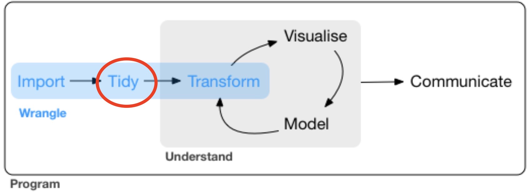
Figure 6.2: Tidy!
In this week’s session, you will learn that tidy data sets obey three rules:
- Variables are represented in columns
- Observations are represented as rows
- Values are contained within cells
For example, consider an study where researchers are interested in the effect of time of day (morning vs. evening) and stimulus type (words vs. images) on memory performance. 5 Participants were tested in both the morning and the afternoon, and had to learn lists of words and images. Participants then had to recall what they had learned, and the percent correct was used as the measure of memory accuracy.
Here’s one way you might store the data in R:
## # A tibble: 5 × 5
##   participant morning_words morning_images evening_words evening_images
##         <int>         <dbl>          <dbl>         <dbl>          <dbl>
## 1           1          96.6           80.8          78.3           97.6
## 2           2          97.5           89.5          88.8           99.1
## 3           3          71.4           65.4          97.4           64.7
## 4           4          93.2           86.3          70.2           79
## 5           5          85.7           88.2          78.5           82.4
As you will come to learn, this data is not tidy because it violates two of the three rules:
- Variables are represented in columns: FALSE. Columns instead represent individual levels of the experiment design rather than variables.
- Observations are represented as rows: FALSE. Each participant has 4 observations, but the rows represent each individual participant rather than individual observations.
- Values are contained within cells: (Sort of) TRUE. But ideally we should only have one column that represents values.
Here is exactly the same data, but in a tidy format:
## # A tibble: 20 × 4
##    participant time_of_day stimulus_type memory_score
##          <int> <chr>       <chr>                <dbl>
##  1           1 morning     words                 96.6
##  2           1 morning     images                80.8
##  3           1 evening     words                 78.3
##  4           1 evening     images                97.6
##  5           2 morning     words                 97.5
##  6           2 morning     images                89.5
##  7           2 evening     words                 88.8
##  8           2 evening     images                99.1
##  9           3 morning     words                 71.4
## 10           3 morning     images                65.4
## 11           3 evening     words                 97.4
## 12           3 evening     images                64.7
## 13           4 morning     words                 93.2
## 14           4 morning     images                86.3
## 15           4 evening     words                 70.2
## 16           4 evening     images                79
## 17           5 morning     words                 85.7
## 18           5 morning     images                88.2
## 19           5 evening     words                 78.5
## 20           5 evening     images                82.4
This now obeys the three rules:
- Variables are represented in columns: TRUE. The columns
time_of_dayandstimulus_typeare variables in our data. - Observations are represented as rows: TRUE. Each row now represent individual observations, and the columns represent what level of the variables the observation had. For example, in row 1 we see the observation for
participant 1in themorningwhen learningwords. - Values are contained within cells: TRUE. We now have the column
memory_scorewhich tracks the value for each observation.
This week we are going to learn how to wrangle your data to get it into a tidy format. Let’s get stuck in:
6.3 Workshop Exercises
Import the
pepsi_challenge.csvdata from the Open Science Framework, and save it to an object calledpepsi_data. This is fake data from a “Pepsi Challenge”. 100 participants were asked to try three separate drinks, and rate each drink out of 10 (with 10 being the best score). Little did the participants know that one of the drinks was Pepsi, one was Coca-Cola, and the other was a supermarket’s own brand cola. Wrangle this data into long format, saving the result into an object calledlong_data.Although not the main focus of this week’s learning, use your skills from last week to show the mean rating per drink across participants.
Using pipes, go from the original data (pepsi_data) to a plot of the mean ratings per drink on a scatter plot.
- (Note, a scatter plot really isn’t the best type of visualisation for this, but it’s all that we have learned so far!)
Import the
time_stimtype.csvdata from the Open Science Framework, and save it to an object calledmemory_data. This is fake data from the memory and stimulus type experiment mentioned at the beginning of this chapter. Wrangle this data into long format, saving the result into an object calledlong_data.- Hint: Note that the variable names are separated in the columns by an underscore (“_“). When you use the
pivot_longerfunction, you may want to add the argumentnames_sep = "_"to tell R that the variable names are separated by an underscore.
- Hint: Note that the variable names are separated in the columns by an underscore (“_“). When you use the
Import the
stroop_data.csvfile from the Open Science Framework storing to an object calledstroop_data.- This is data from a classic Stroop test. Response times are typically slower on incongruent trials (where the colour of the text and the word do not match) than on congruent trials (where the colour of the text and the word do match).
- The data shows response times (in milliseconds) for 30 participants (coded in the
idcolumn). Each participant had 500 congruent trials and 500 incongruent trials.
5a. What was the mean response time per participant, per level of congruency?
5b. Which participant had the slowest overall mean response time?
5c. Transform the data into wide format so that for each participant there is a column showing mean response time for congruent trials and another column showing mean response time for incongruent trials. Each row should be a unique participant.
- Hint: You will need to first perform the same code as you did for 5a to get the mean RT per participant per congruency level and then make use of the
pivot_wider()function. - Here’s what it should look like in the end:
## # A tibble: 30 × 3
## # Groups:   id [30]
##       id congruent incongruent
##    <int>     <dbl>       <dbl>
##  1     1      614.        651.
##  2     2      637.        671.
##  3     3      630.        678.
##  4     4      410.        445.
##  5     5      469.        522.
##  6     6      371         390.
##  7     7      572.        601.
##  8     8      511.        507.
##  9     9      714.        730.
## 10    10      427.        463.
## # … with 20 more rows
5d. The “Stroop Effect” is determined as the mean response time for incongruent trials minus the mean response time for congruent trials. Calculate the Stroop Effect for each participant in the data. * Hint: You may need to repeat what you did in 5c, but then you need just one more step…