9 Week 9: Reproducible Reports with R Markdown — Part 1
9.1 Overview
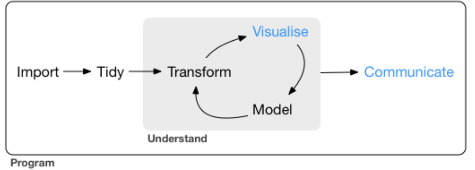
Figure 9.1: Creating your first markdown document!
In the next 2 weeks we are going to learn how to use R Markdown, which enables you to produce reproducible reports of your analysis that combines text, code, and output of your analysis (such as transformed data and plots). Such markdown documents are incredibly useful for communicating your analysis to others (and can be useful as a communication to future you!).
Here is a simple R markdown file:
---
title: "Markdown Example"
author: "Your Name"
date: "March 2023"
output: pdf_document
---

## R Markdown

This is an example R Markdown document.

It combines **commentary** (i.e., plain text), **analysis code**, and the **output** of any
code (e.g., showing data and plots).

You can embed R code into your documents by including "chunks" like this:

```{r}
# load the tidyverse
library(tidyverse)

# show the diamonds data set (part of the tidyverse)
diamonds
```

You can also embed plots into the report, for example:

```{r}
data_snippet <- diamonds %>%
  filter(clarity == "VVS1")

ggplot(data = data_snippet, aes(x = carat, y = price)) +
  geom_point() +
  geom_smooth() +
  labs(x = "Carat of Diamond",
       y = "Price (USD)")
```
We will learn what is going on in this file this week, and you will have plenty of time to practice using them. Your answers to the R assessment for this module will be written using an R markdown document.
9.2 Before you Do Anything Else…
Before we do any reading this week, I just want to make sure that everything runs as expected on your computer. Everything should be pre-installed together with R Studio, but if not I want to catch this early so I can help you get everything installed. We are going to create a template markdown document and see if it runs.
To do this, create a new project (give it any name you wish) in a folder of your choosing. In previous weeks, you’ve used scripts to write your code by going to File > New File > R Script inside R Studio. Today, however, go to File > New File > R Markdown..., and you will see the following dialogue box appear:
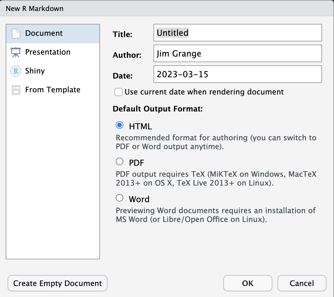
Figure 9.2: Creating your first markdown document!
Enter your name and any title you please into the relevant boxes. Leave everything else as it is, and click OK. A template R markdown file should now open in R Studio. Save this file to your project folder. After this, click on the Knit button in R Studio toolbar.
If everything runs OK, a webpage should appear with the title you gave it and your name; below it there should be some text, data, and a plot.
This is an html version of your R Markdown file! We can also create a PDF and a Word document of this file, which we will try now. Click on the little arrow next to the Knit button in the R Studio toolbar. When you do this, the following options menu should appear:
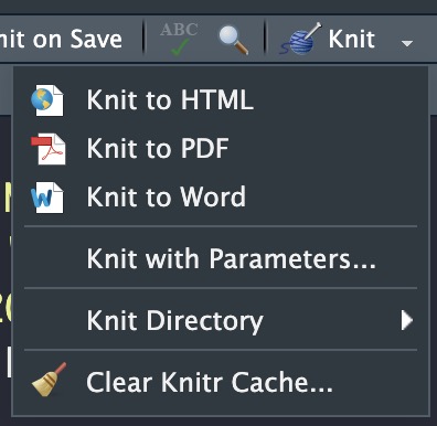
Try the following (in this order): * First, try and “Knit to Word”. If this works, a new Microsoft Word document should open with the contents of your file showing. * Second, try and “Knit to PDF”. If this works—you guessed it—a new PDF file should open with the contents of your file showing.
If any of the above do not work, contact me ASAP! When contacting me, try and take a screenshot of any errors you are getting.
9.3 Reading
If the above has worked, you can move on to this week’s reading. We are going back to the R4DS book, but we are only going to use a tiny portion of the relevant chapter this week. Therefore, only read the following sections:
- 27.1 Introduction to R Markdown
- 27.1.1 Prerequisites, although this should have been covered by the above.
- 27.2 R Markdown basics
- 27.3 Text formatting with Markdown
- ONLY 27.4 (i.e., don’t worry about going into 27.4.1 etc…)