4 Week 4: Getting Organised, Scripts, & Data Handling
4.1 Overview
This week is all about getting organised. Who doesn’t love getting organised?

Figure 4.1: Marie Kondo would love this chapter.
So far, you have just been entering R code into the console one command at a time. Whilst this is useful whilst you are learning how to use R, pretty soon this is going to be unsustainable because you need to write multiple lines of code. As the number of lines of code you need to write increases, it becomes more and more important for reproducibility that you keep a record of the commands you have used. This is where scripts come in handy: They are a single file which contains a record of all commands you use to conduct a piece of data analysis.
We will also cover how to get organised with the files you are using by introducing you to the use of projects in R Studio. These are self-contained environments that keep all relevant files associated with your analysis in one place. And pretty soon you will have plenty of files associated with your analysis: You will have raw data files, new post-processing data files, analysis scripts, saved data visualisations etc. For simple analyses, projects are likely overkill, but it’s good practice to start using them now so that when they become necessary they are second-nature.
We will also discuss how to import and export data. Obviously, without data no analysis can happen. So far we have been using data built-in to R packages; whilst these are great for playing around, your learning will likely accelerate as you start using data more familiar to you. You will practice importing data files created by me, but I encourage you to start importing your own data and playing around with it!
4.2 Reading
- Chapter 6 from R4DS
- This introduces you to scripts.
- Note that the example code in this chapter use functions introduced in Chapter 5, which is a chapter I have not (yet!) asked you to read. So don’t worry at this stage that you don’t know what the code does.
- Practice using scripts to enter some of the commands you have learned over the previous weeks.
- Chapter 8 from R4DS
- This introduces you to projects.
- The important material really starts in Section 8.4., but the preceding material in the chapter provides some important context.
- Read the bespoke material below about importing & exporting data.
- R4DS does have chapters on this topic, but they are buried in denser material less relevant to an introductory course.
Tip. In scripts, it is strongly recommend that you add comments to describe what the code is doing. This is useful both as a reminder to your future-self (it’s easy to forget what the code does when you revisit an old script!) but also to describe to other researchers what the code does (thus enhancing reproducibility).
In R scripts, any line beginning with a # symbol is a comment and is not evaluated by R. See below for an example!
# This line is a comment. Hello, future me!
# The line below this is NOT a comment.
x <- 4
4.2.1 Handling Data
In this section we will discuss how to handle data that is contained on your own computer that you have either created yourself or have downloaded from elsewhere. For this section, please create a new project in a folder (AKA directory) somewhere on your computer. Then create a new script in that project folder. All of the commands shown in this section should be entered into your script, and then executed either one-by-one, or all at once. As with all scripts you will write on this course, the first thing you should do is load the tidyverse package.
library(tidyverse)4.2.1.1 Data formats
For the majority of this course, we will be using .csv files (“comma separated values” files). These are similar to Excel spreadsheets but are saved in a way such that they can be read by a wider array of software programs. Saving your data in non-proprietary formats is just one more way you can make your research more open and reproducible, because more people will be able to access it.
4.2.1.2 Importing data
I will provide you a few data sets to play around with. These can be accessed on my Open Science Framework account which can be found here: https://osf.io/z5tg2/.
For the first example, we will use the gorilla_bmi.csv data file. Please download this from the Open Science Framework and place it into your project folder. You can double-click on this file to open it in Excel (or your favourite database program) if you wish. But in order to open this file within R, we use the read_csv() function from the tidyverse package.
Tip. Remember to find out more about a function you can use the ? helper command. So, in this case you could type ?read_csv into the console to find out more about the function we are going to use. You will read that the function accepts many arguments; however, we are going to use just the file argument. We may use some more advanced features of this function later in the module.
When importing data, it’s essential that you save the data to an object otherwise you won’t be able to access the data. For now, you can just call the object data if you want, but as you start to handle multiple data files in the same project you may want to come up with a more unique object name for each data set (for example, maybe gorilla_bmi_data).
So to import your data, use the following:
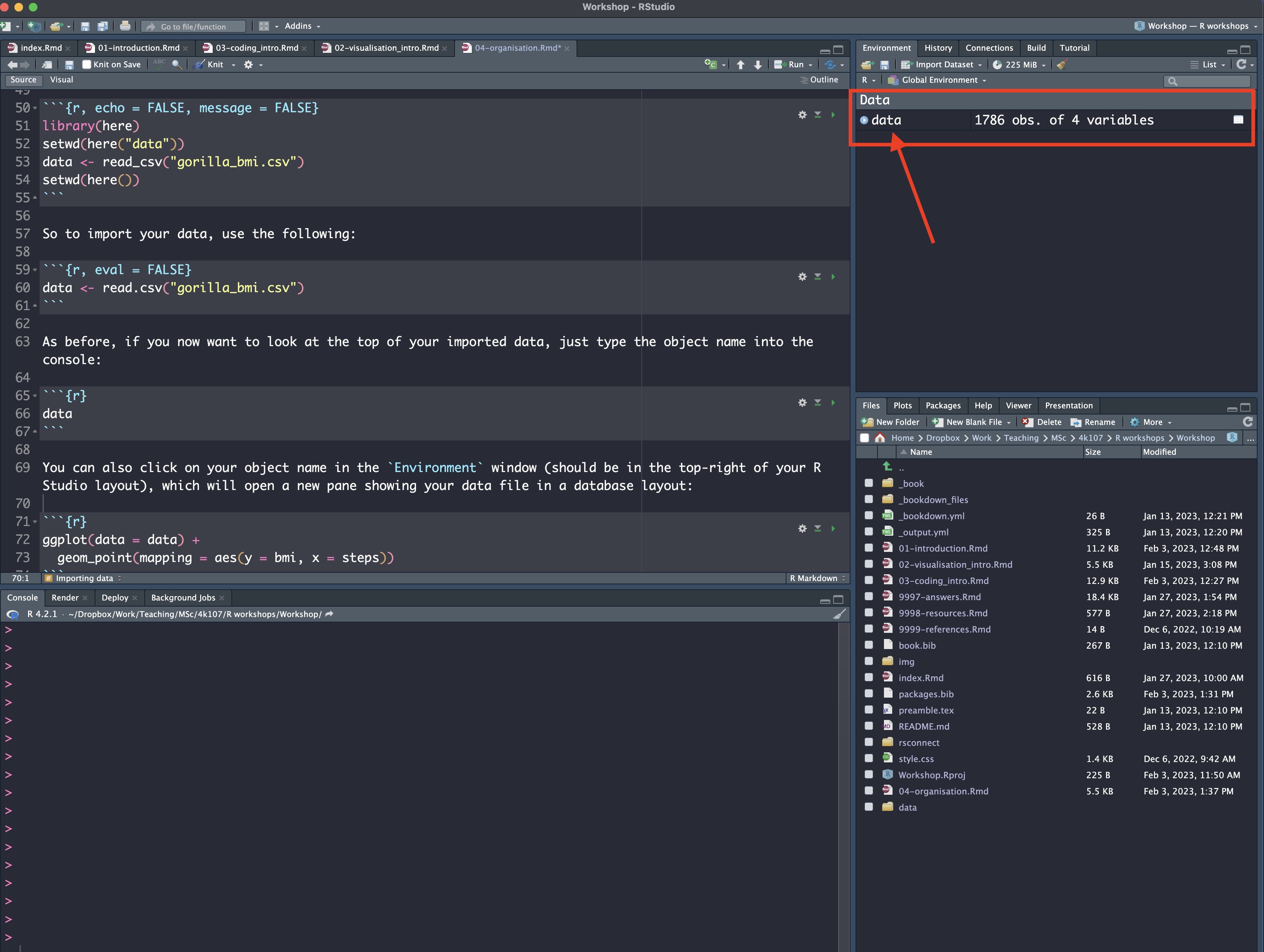
data <- read_csv("gorilla_bmi.csv")As before, if you now want to look at the top of your imported data, just type the object name into the console:
data## # A tibble: 1,786 × 4
## id steps bmi gender
## <dbl> <dbl> <dbl> <chr>
## 1 1 15000 16.9 male
## 2 2 15000 16.9 male
## 3 6 14861 16.8 male
## 4 7 14861 16.8 male
## 5 8 14699 17.3 male
## 6 10 14560 20.5 male
## 7 11 14560 20.6 male
## 8 13 14560 20.5 male
## 9 17 14560 20.4 male
## 10 18 14560 20.4 male
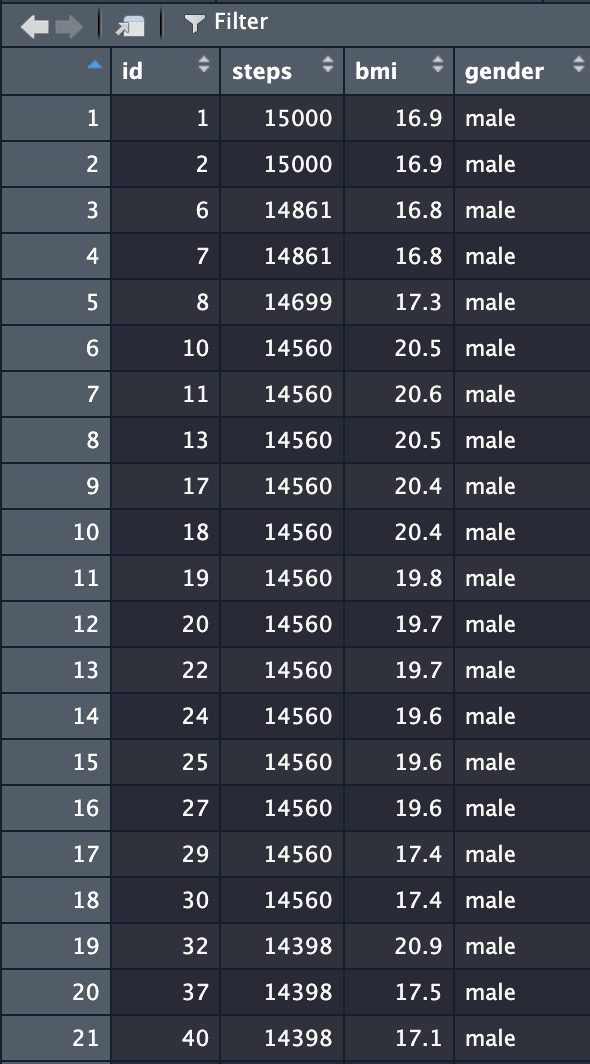
## # … with 1,776 more rowsYou can also click on your object name in the Environment window (should be in the top-right of your R Studio layout), which will open a new pane showing your data file in a database layout:
4.2.1.3 Exporting data
Exporting data from R is useful for saving your data after some processing has occurred. For example, you may have removed some outliers from your data or transformed some variables before conducting your final visualisation / analysis. As your final data has been altered from the raw data, it’s useful to save this final data so that others can access it.
As we haven’t learned how to process our data much yet, we will practice exporting data using some of the built-in data sets in the tidyverse. We will use the write_csv() function from the tidyverse. This requires two arguments: (1) the data we would like to save, and (2) the name we would like the new file to have. Let’s practice this using the Titanic data that is built into R:
titanic_data <- TitanicAgain we have saved it to a new object, but this time we’ve used a slightly more informative name for the object. Now, to save this data to our project folder, we do the following:
write_csv(titanic_data, file = "titanic_data.csv")Here, we have told the function that we want to save the titanic_data object, and we want to give it the name titanic_data.csv). Once you have executed this command, you should see a new .csv file in your project folder with the name you provided it.
4.2.1.4 Exporting plots
Later in the module I will show you how to save any plots you create using ggplot with code, but for now just note that you can save any plots you create directly from within R Studio. First let’s create a plot using built-in data:
ggplot(data = mpg) +
  geom_point(mapping = aes(x = displ, y = hwy))
In the window that shows your plot, click on the “Export” button (see Figure below:)
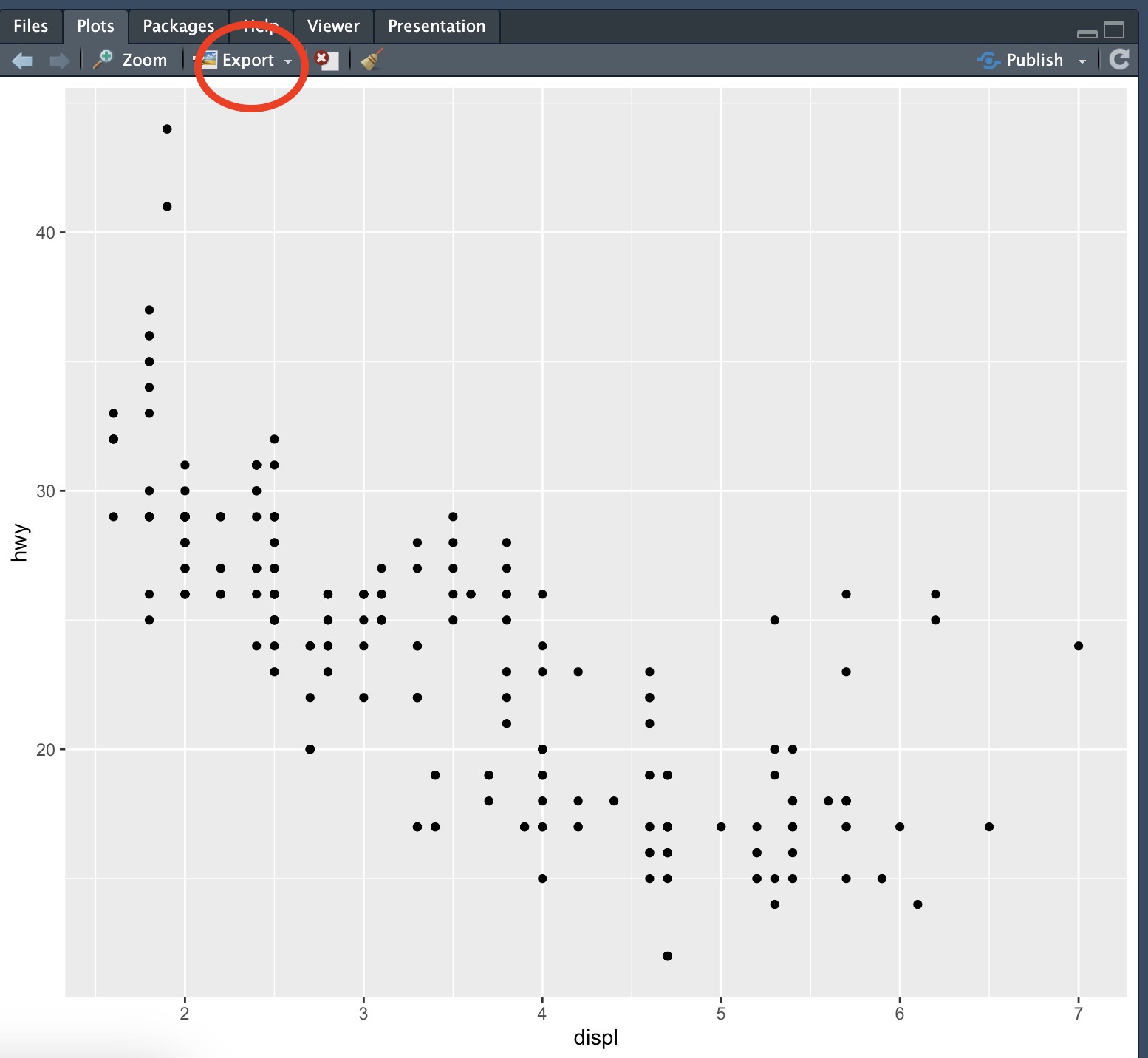
This gives you the option to either save the plot as an image (a .png file) or as a PDF file. Usually you should prefer the former, but it’s up to you. Once you’ve chosen, the plot will show in a new window. Note that you can resize the plot as you so wish using the tab in the bottom-right corner of the screen (or you can manually enter the desired width and height in the relevant box):
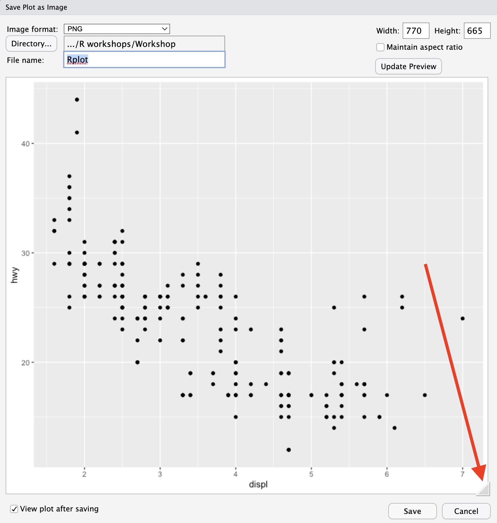
Once the plot is sized to your satisfaction, click save. The requested file should now appear in your project folder.
4.3 Workshop Exercises
Create a new script called
gorillaand write code that achieves the following:- Import the
gorilla_bmi.csvdata from the OSF - Create a scatter plot showing steps on the x-axis and bmi on the y-axis
- Save the image as a .png with the name
gorilla_plot. - Do you notice anything?
- Import the
Save this plot using the method described in this week’s reading.
Have a look at the help file for the
ggsavefunction. How might you use this function to save the plot you’ve created with the following characteristics?- file name equal to
gorilla_bmi_ggsave.png - Width of the plot should be 6 inches
- Height of the plot should be 5 inches
- file name equal to
Writing clear R code is important, especially now you are starting to write scripts. It must be readable to you, but also to other researchers for it to be reproducible. With reference to the tidyverse R style guide, re-write the following code into a well-formatted script. (Don’t worry if you don’t know what everything does; we are just looking to make sure we are using a clear style. Don’t forget the importance of good commenting!).
library(tidyverse)

# data
D = diamonds

# filter the data to only show diamonds with "SI2" clarity
FilteredData <- filter(D, clarity == "SI2")

# plot 1
ggplot(data=FilteredData) + geom_point(aes(x=carat, y=price))

# another plot
ggplot(data=FilteredData) + geom_point(aes(x=carat, y=price,color=depth))