Chapter 1 关于R语言

本文是统计计算的课程笔记整理，主要采用R语言编程。

R是一个免费开源的用于统计计算和作图的语言和软件环境，它提供了广泛的统计工具和灵活高质量的图形工具，其功能可以通过添加package来扩充。R的官方网站为 R Project Website，该网站包含R在各种操作系统下的安装文件、R的帮助文档包括一些免费的书籍等。

R是一种解释性语言，不必像C之类的编译语言首先要构成一个完整的程序形式。当R运行时，所有变量、数据、函数及结果都以对象（object）的形式存在计算机的活动内存中，并冠有相应的名字代号。我们可以通过用一些运算符（如算术、逻辑、比较等）和一些函数（其本身也是对象）来对这些对象进行操作。

1.1 数据结构（Data Structure）

R中的数据结构可以按其维数（1d、2d、nd）和同质性（所有元素必须属于同一类型）来区分，常见的有：

	同质的	异质的
1d	原子向量（Atomic vector）	列表（List）
2d	矩阵（Matrix）	数据框（Data frame）
nd	数组（Array）

利用str()函数可以得到对象的数据结构。

str(list(list(1,2), c(3,4)))

## List of 2
##  $ :List of 2
##   ..$ : num 1
##   ..$ : num 2
##  $ : num [1:2] 3 4

1.1.1 向量（Vector）

向量是R中的基本对象，主要分为原子向量（Atomic vector）和列表（List）两种。

类型：通过typeof()可以得到向量的类型；
长度：通过length()可以得到向量中有多少元素；
属性：通过attributes()可以得到向量外在的附加属性。

1.1.1.1 原子向量（Atomic vector）

可以使用函数c()或seq()等来创建，它可以是数值型、字符型和逻辑型，缺失用NA表示。

dbl_var <- c(1, 2.5, 4.5)
is.integer(dbl_var)

## [1] FALSE

int_var <- c(1L, 6L, 10L)
typeof(int_var)

## [1] "integer"

log_var <- c(TRUE, FALSE)
is.atomic(log_var)

## [1] TRUE

chr_var <- c("these are", "some strings", NA)
length(chr_var)

## [1] 3

当使用c()来创建时，不同类型的元素同时在向量内时，存在如下的次序关系：

logical < integer < double < character < list

str(c("a", 1))

##  chr [1:2] "a" "1"

str(c(FALSE, 1L, list(1)))

## List of 3
##  $ : logi FALSE
##  $ : int 1
##  $ : num 1

可以看到第一个结果被强制转换为了字符型，第二个结果被强制转换为了列表。

1.1.1.2 列表（List）

相比于原子向量，列表的元素允许有不同类型的元素存在。

str(list(1:3, "a", c(TRUE, FALSE), c(2.3, 5.9)))

## List of 4
##  $ : int [1:3] 1 2 3
##  $ : chr "a"
##  $ : logi [1:2] TRUE FALSE
##  $ : num [1:2] 2.3 5.9

此外，列表中允许嵌套列表，即存在递归的结构。

x <- list(list(1, 2), c(3, 4))
str(x)

## List of 2
##  $ :List of 2
##   ..$ : num 1
##   ..$ : num 2
##  $ : num [1:2] 3 4

is.recursive(x)

## [1] TRUE

y <- c(list(1, 2), c(3, 4))
str(y)

## List of 4
##  $ : num 1
##  $ : num 2
##  $ : num 3
##  $ : num 4

is.recursive(y)

## [1] TRUE

使用unlist()函数可以将列表转换为原子向量，当然利用c()也可以。

str(unlist(x))

##  num [1:4] 1 2 3 4

1.1.2 属性（Attribute）

前面我们讲通过attributes()可以得到附加属性，那么如何添加属性呢？attr()帮助我们解决这一问题。

y <- 1:10
attr(y, "my_attribute") <- "This is a numeric vector"
str(y)

##  int [1:10] 1 2 3 4 5 6 7 8 9 10
##  - attr(*, "my_attribute")= chr "This is a numeric vector"

attributes(y)

## $my_attribute
## [1] "This is a numeric vector"

此外，我们利用structure()在构建新的对象时也可以直接加属性。

structure(1:10, my_attribute = "This is a numeric vector")

##  [1]  1  2  3  4  5  6  7  8  9 10
## attr(,"my_attribute")
## [1] "This is a numeric vector"

1.1.2.1 因子（Factor）

属性的一种重要应用是定义因子。因子是一个向量，但是它的元素只能是特定的一些值，通常被用来存储分类数据。

x <- factor(c("a", "b", "b", "a"))
x

## [1] a b b a
## Levels: a b

class(x)

## [1] "factor"

levels(x)

## [1] "a" "b"

对于不在level中的值，我们不能进行赋值操作，系统会将其置为缺失值NA。

x[2] <- "c"

## Warning in `[<-.factor`(`*tmp*`, 2, value = "c"): invalid factor level, NA generated

## [1] a    <NA> b    a   
## Levels: a b

有时候我们从文件中读取数据时，可能会出现错误将向量误认为因子的情况，可以借助stringsAsFactors参数予以解决（最新版的默认参数已设定为FALSE，大部分情况不会出错），参考下面两个例子。

a <- read.table(text = "A B\nNA 0\n1.2 1\nNN 2", sep = "", head = TRUE)
str(a)

## 'data.frame':    3 obs. of  2 variables:
##  $ A: chr  NA "1.2" "NN"
##  $ B: int  0 1 2

as.numeric(a[,1])

## Warning: 强制改变过程中产生了NA

## [1]  NA 1.2  NA

b <- read.table(text = "A B\nNA 0\n1.2 1\nNN 2", sep = "", head = TRUE,
                stringsAsFactors = TRUE)
str(b)

## 'data.frame':    3 obs. of  2 variables:
##  $ A: Factor w/ 2 levels "1.2","NN": NA 1 2
##  $ B: int  0 1 2

as.numeric(b[,1])

## [1] NA  1  2

从上面第二个示例中可以看到，因子在系统内实际上是以连续的整数存储。在实际问题中，我们可能还需要改变因子的水平（levels），即背后的数字大小，可以通过levels()或在创建因子时对参数levels做修改来实现。

f1 <- factor(letters)
f1

##  [1] a b c d e f g h i j k l m n o p q r s t u v w x y z
## Levels: a b c d e f g h i j k l m n o p q r s t u v w x y z

levels(f1) <- rev(levels(f1))
f1

##  [1] z y x w v u t s r q p o n m l k j i h g f e d c b a
## Levels: z y x w v u t s r q p o n m l k j i h g f e d c b a

f2 <- rev(factor(letters))
f2

##  [1] z y x w v u t s r q p o n m l k j i h g f e d c b a
## Levels: a b c d e f g h i j k l m n o p q r s t u v w x y z

f3 <- factor(letters, levels = rev(letters))
f3

##  [1] a b c d e f g h i j k l m n o p q r s t u v w x y z
## Levels: z y x w v u t s r q p o n m l k j i h g f e d c b a

1.1.3 矩阵（Matrix）与数组（Array）

通过对原子向量添加维数dim()操作可以的得到一个多维的数组，特别地，矩阵是二维数组。

# matrix
a <- 1:6
dim(a) <- c(3, 2)
a

##      [,1] [,2]
## [1,]    1    4
## [2,]    2    5
## [3,]    3    6

# array
b <- 1:12
dim(b) <- c(2, 3, 2)
b

## , , 1
## 
##      [,1] [,2] [,3]
## [1,]    1    3    5
## [2,]    2    4    6
## 
## , , 2
## 
##      [,1] [,2] [,3]
## [1,]    7    9   11
## [2,]    8   10   12

当然，也可以直接利用matrix()或array()直接构建，下面代码与上面等价。

a <- matrix(1:6, nrow = 3, ncol = 2)
b <- array(1:12, c(2, 3, 2))

如果要对不同的维度添加对应的名字，可以通过rownames，colnames和dimnames操作。

rownames(a) <- c("A", "B", "C")
colnames(a) <- c("a", "b")
a

##   a b
## A 1 4
## B 2 5
## C 3 6

dimnames(b) <- list(c("one", "two"), c("a", "b", "c"), c("A", "B"))
b

## , , A
## 
##     a b c
## one 1 3 5
## two 2 4 6
## 
## , , B
## 
##     a  b  c
## one 7  9 11
## two 8 10 12

需要说明的是，对列表也可以添加维度来得到列表矩阵或列表数组。

l <- list(1:3, "a", TRUE, 1.5)
dim(l) <- c(2, 2)
l

##      [,1]      [,2]
## [1,] Integer,3 TRUE
## [2,] "a"       1.5

关于一些数据结构的合并，也有以下几种方式：

c()：合并向量；
cbind()，rbind()：合并矩阵；
abind::abind()：合并数组。

值得说明的是，合并的结果遵循强制转换原则，而且这些操作很费时间和空间。

a <- c(1, 2, 3); b <- c("1", "2", "3")
c(a, b)

## [1] "1" "2" "3" "1" "2" "3"

a <- matrix(1:4, nrow = 2, ncol = 2)
b <- matrix(5:8, nrow = 2, ncol = 2)
cbind(a, b)

##      [,1] [,2] [,3] [,4]
## [1,]    1    3    5    7
## [2,]    2    4    6    8

rbind(a, b)

##      [,1] [,2]
## [1,]    1    3
## [2,]    2    4
## [3,]    5    7
## [4,]    6    8

a <- array(1:8, c(2, 2, 2))
b <- array(letters[1:8], c(2, 2, 2))
abind::abind(a, b)

## , , 1
## 
##      [,1] [,2]
## [1,] "1"  "3" 
## [2,] "2"  "4" 
## 
## , , 2
## 
##      [,1] [,2]
## [1,] "5"  "7" 
## [2,] "6"  "8" 
## 
## , , 3
## 
##      [,1] [,2]
## [1,] "a"  "c" 
## [2,] "b"  "d" 
## 
## , , 4
## 
##      [,1] [,2]
## [1,] "e"  "g" 
## [2,] "f"  "h"

1.1.4 数据框（Data-Frame）

数据框是一列等长的向量组成的列表，它具有矩阵和列表的共同性质。

df <- data.frame(x = 1:3, y = c("a", "b", "c"))
c(typeof(df), class(df))

## [1] "list"       "data.frame"

str(df)

## 'data.frame':    3 obs. of  2 variables:
##  $ x: int  1 2 3
##  $ y: chr  "a" "b" "c"

由于数据框本质上是列表，因此我们可以构建元素为列表的数据框。

dfl <- data.frame(x = 1:3, y = I(list(1:2, 1:3, 1:4)))
str(dfl)

## 'data.frame':    3 obs. of  2 variables:
##  $ x: int  1 2 3
##  $ y:List of 3
##   ..$ : int  1 2
##   ..$ : int  1 2 3
##   ..$ : int  1 2 3 4
##   ..- attr(*, "class")= chr "AsIs"

或者更极致的，直接构建元素为矩阵的数据框。

dfm <- data.frame(x = 1:3, y = I(matrix(1:9, nrow = 3)))
str(dfm)

## 'data.frame':    3 obs. of  2 variables:
##  $ x: int  1 2 3
##  $ y: 'AsIs' int [1:3, 1:3] 1 2 3 4 5 6 7 8 9

虽然上述这些操作可行，但是实际问题中，我们还是使得数据框中每一列都是一个原子向量。

1.2 子集操作（Subsetting）

子集操作往往是实践项目中一个很重要的事情，因为我们有时并不是在整个数据集上进行分析。在R中，不同的操作在不同数据类型上的表现不尽相同。

1.2.1 数据类型（Data Type）

1.2.1.1 向量

一般使用[就可以实现子集操作，下面以原子向量为例（列表操作类似）。

x <- c(2.1, 4.2, 3.3, 5.4)
# positive integers
x[c(3, 1)]

## [1] 3.3 2.1

# real number are silently truncated to integers
x[c(2.1, 2.9)]

## [1] 4.2 4.2

# negative integers
x[-c(3, 1)]

## [1] 4.2 5.4

# logical vectors (with NA)
x[c(TRUE, TRUE, NA, FALSE)]

## [1] 2.1 4.2  NA

# logical vectors from operator
x[x > 3]

## [1] 4.2 3.3 5.4

1.2.1.2 矩阵与数组

也是通过[就可以实现，不过这里是多维的操作。

x <- matrix(1:9, nrow = 3, ncol = 3)
colnames(x) <- c("A", "B", "C")
# blank means keep all rows or all columns
x[1:2, ]

##      A B C
## [1,] 1 4 7
## [2,] 2 5 8

# with names
x[c(TRUE, FALSE, TRUE), c("C", "B")]

##      C B
## [1,] 7 4
## [2,] 9 6

# column-major order subsetting
x[c(1, 5, 8)]

## [1] 1 5 8

1.2.1.3 数据框

可以使用[，也可以使用$实现。

df <- data.frame(x = 1:3, y = 3:1, z = letters[1:3])
# with [ and $
df[df$x == 2, ]

##   x y z
## 2 2 2 b

# with numbers
df[c(1, 3), ]

##   x y z
## 1 1 3 a
## 3 3 1 c

# with names (two examples)
df[c("z", "x")]

##   z x
## 1 a 1
## 2 b 2
## 3 c 3

df[, c("z", "x")]

##   z x
## 1 a 1
## 2 b 2
## 3 c 3

注意如果只选一列的话两个操作并不是等价的。

str(df["x"])

## 'data.frame':    3 obs. of  1 variable:
##  $ x: int  1 2 3

str(df[, "x"])

##  int [1:3] 1 2 3

1.2.1.4 S3对象和S4对象

S3对象包括向量、数组等这些，用前面所述方式就可以实现子集操作，而S4对象则需要@（与$等价）或slot()（与[[等价）操作来实现。

1.2.2 操作算子（Subsetting Operator）

这里我们介绍另外两个操作算子[[和$。

对于[[而言，当其作用在列表上时，可以得到对应的元素，而[只能得到一个列表。

x <- list(a = 1, b = 2)
str(x[1])

## List of 1
##  $ a: num 1

str(x[[1]])

##  num 1

对于$而言，其往往作用在数据框上，是一种更为简化的算子，比如df$x就等价于df[["x", exact = FALSE]]。不过需要注意的是，如果将列名存在变量里时，就不能使用上述简化了。

df <- data.frame(x = 1:3, y = letters[1:3])
var <- "x"
df$var

## NULL

df[[var]]

## [1] 1 2 3

在R中，关于操作算子还有两个重要原则需要介绍：简化（simplify）与保留（preserve）。

简化（Simplify）：子集操作后返回结果的最简可能数据结构。
保留（Preserve）：子集操作后返回结果的结构。

	简化（Simplify）	保留（Preserve）
向量	`x[[1]]`	`x[1]`
因子	`x[1:4, drop = T]`	`x[1:4]`
数组	`x[1, ]`或`x[, 1]`	`x[1, , drop = F`或`x[, 1, drop = F]`
数据框	`x[, 1]`或`x[[1]]`	`x[, 1, drop = F]`或`x[1]`

# atomic vector: remove names
x <- c(a = 1, b = 2)
x[1]

## a 
## 1

x[[1]]

## [1] 1

# factor: drops any unused levels
z <- factor(c("a", "b"))
z[1]

## [1] a
## Levels: a b

z[1, drop = T]

## [1] a
## Levels: a

# array: drops dimension if possible
a <- matrix(1:4, nrow = 2, ncol = 2)
a[1, , drop = F]

##      [,1] [,2]
## [1,]    1    3

a[1, ]

## [1] 1 3

# data frame: return vector instead of data frame if possible
df <- data.frame(a = 1:2, b = 1:2)
str(df[1])

## 'data.frame':    2 obs. of  1 variable:
##  $ a: int  1 2

str(df[[1]])

##  int [1:2] 1 2

本质上，这些操作算子都是为了应用上的方便，比如随机抽样、排序、条件取值等等。

# sample (bootstrap)
df <- data.frame(x = rep(1:3, each = 2), y = 6:1, z = letters[1:6])
df[sample(nrow(df)),]

##   x y z
## 2 1 5 b
## 6 3 1 f
## 1 1 6 a
## 3 2 4 c
## 5 3 2 e
## 4 2 3 d

# order
df[order(df$y), ]

##   x y z
## 6 3 1 f
## 5 3 2 e
## 4 2 3 d
## 3 2 4 c
## 2 1 5 b
## 1 1 6 a

# condition
df[df$x == 2, ]

##   x y z
## 3 2 4 c
## 4 2 3 d

df[which(sample(6) < 4), ]

##   x y z
## 1 1 6 a
## 3 2 4 c
## 6 3 1 f

1.3 函数编程（Functional Programming）

R中的所有函数都有以下三个部分：

主体（body）部分：函数内的代码；
形参（formals）部分：调用函数时的形式参数列表；
环境（environment）部分：函数变量在内存中的映射位置。

f <- function(x) { x^2 }
f

## function(x) { x^2 }
## <environment: 0x7fb84a9662a8>

formals(f)

## $x

body(f)

## {
##     x^2
## }

environment(f)

## <environment: 0x7fb84a9662a8>

此外，在R中所有的运算符都是一种函数调用，只不过这种函数调用已经通过R底层写好了。

x <- 10; y <- 5
`+`(x, y)  # same as `x + y`

## [1] 15

1.3.1 循环函数：`lapply`的朋友们

下面介绍lapply家族的一些函数。

lapply(x, f, ...)：对列表x中的每个元素作用函数f，返回作用后的结果，...取决于函数的参数。
sapply(x, f, ..., simplify = TRUE, USE.NAMES = TRUE)：是lapply函数更加精细的版本（如果最后两个参数均为FALSE则效果与lapply相同），可以返回向量、矩阵或数组（simplify = "array"）。
vapply(x, f, f.value, ..., USE.NAMES = TRUE)：与sapply类似，但是可以预定义返回值的类型。

add <- function(x, y) x + y
sapply(1:5, add, 3)

## [1] 4 5 6 7 8

# same as above
sapply(1:5, `+`, 3)

## [1] 4 5 6 7 8

my_summary <- function(x) {
  funs <- c(mean, median, sd, mad, IQR)
  sapply(funs, function(f) f(x, na.rm = TRUE))
}
df <- data.frame(replicate(6, sample(c(1:10, NA), 10, rep = T)))
vapply(df, my_summary, FUN.VALUE = c(mean = 0, median = 0, sd = 0, mad = 0, IQR = 0))

##              X1       X2       X3       X4       X5       X6
## mean   5.700000 5.142857 5.500000 6.444444 6.555556 5.900000
## median 7.000000 4.000000 5.000000 6.000000 7.000000 7.000000
## sd     2.750757 2.544836 3.205897 2.833333 2.351123 2.960856
## mad    2.965200 2.965200 3.706500 2.965200 1.482600 2.965200
## IQR    3.750000 3.500000 4.500000 3.000000 4.000000 4.000000

对于lapply()而言，函数的参数只能有一个是变化的，不能应用于多个参数均变化的情形，但是Map()或mapply()可以实现，其中后者还可以再添加更多的函数参数。

xs <- list(runif(10), runif(5))
ws <- list(rpois(10, 2) + 1, rpois(5, 2) + 1)
unlist(Map(weighted.mean, xs, ws))

## [1] 0.5920859 0.4563270

mapply(weighted.mean, xs, ws, MoreArgs = list(na.rm = TRUE))

## [1] 0.5920859 0.4563270

如果我们要滚动计算（rolling computation），可以使用rollapply。

rollapply <- function(x, n, f, ...) {
  offset <- trunc(n / 2)
  locs <- (offset + 1):(length(x) - n + offset - 1)
  vapply(locs, function(i) f(x[(i - offset):(i + offset - 1)], ...), numeric(1))
}
rollapply(1:10, 4, mean)

## [1] 2.5 3.5 4.5 5.5 6.5

set.seed(123)
x <- seq(1, 3, length = 100) + rt(100, df = 2) / 3
par(mar = rep(0.1, 4))
plot(x)
lines(rollapply(x, 5, mean), col = 2, lwd = 2)
lines(rollapply(x, 5, median), col = 4, lwd = 2)
legend("topleft", c("mean", "median"), inset = 0.01, col = c(2, 4), lwd = 2)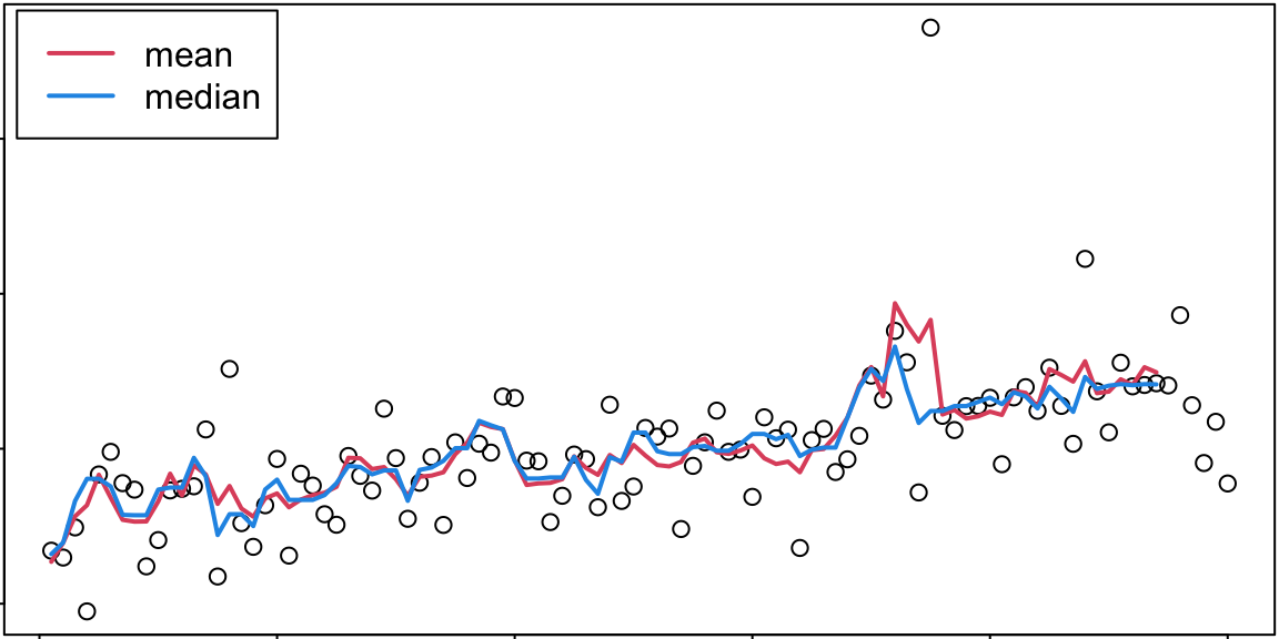

此外，我们要注意到，lapply()函数内部在每次循环都是单独运算的，因此结果的顺序与运算顺序无关。这样的话，我们自然可以实现并行运算，在不同的核上并行运算在进行合并。

library(parallel)
boot_df <- function(x) { x[sample(nrow(x), rep = T), ] }
rsq <- function(model) { summary(model)$r.square }
boot_lm <- function(i) {
  boot_data <- boot_df(mtcars)
  rsq(lm(mpg ~ wt + disp, data = boot_data))
}
n <- 1000
system.time(lapply(1:n, boot_lm))

##    user  system elapsed 
##   1.013   0.014   1.042

system.time(mclapply(1:n, boot_lm, mc.cores = 4))

##    user  system elapsed 
##   0.828   0.183   0.688

这里明显看到并行计算的效率要更差一些。

1.3.2 矩阵与数组的操作（Manipulating）

apply()是sapply()的在矩阵与数组上的变种，其使用方式基本与sapply()类似。

a <- matrix(1:20, nrow = 5)
apply(a, 1, mean)

## [1]  8.5  9.5 10.5 11.5 12.5

apply(a, 2, mean)

## [1]  3  8 13 18

注意这里第二个参数是MARGIN，其值为1表示按行，2表示按列；这里如果是数组，则值还可以继续增大。

a <- array(1:24, c(2, 2, 3, 4))
apply(a, 1, function(x) apply(x, 1:2, mean))

##      [,1] [,2]
## [1,]    7    8
## [2,]    9   10
## [3,]   11   12
## [4,]   13   14
## [5,]   15   16
## [6,]   17   18

结合前面的rollapply函数可以实现按行滚动作用函数的功能。

df <- matrix(rnorm(50), nrow = 10)
apply(df, 2, function(x) rollapply(x, 4, mean))

##            [,1]       [,2]       [,3]       [,4]       [,5]
## [1,] -0.2026764 -0.3201436 -0.7090623 -0.4417866 -0.4310102
## [2,] -0.2868387 -0.7040940 -0.4153395 -0.3360103 -0.1126131
## [3,] -0.3828942 -1.1426186 -0.6082409 -0.2286206 -0.3891445
## [4,] -0.4065427 -1.1465795 -0.9691028 -0.5557991 -0.3887170
## [5,] -0.1199274 -0.6401807 -1.0850576 -0.1765548  0.6502315

sweep()函数可以清理掉描述性统计量的值。下面这段代码实现了数据的列标准化操作。

x <- matrix(rnorm(20, 0, 10), nrow = 4)
x1 <- sweep(x, 1, apply(x, 1, mean), `-`) # minus the row.mean
x2 <- sweep(x1, 1, apply(x1, 1, sd), `/`) # divide the row.sd
x2 # standardize of x

##             [,1]       [,2]       [,3]       [,4]       [,5]
## [1,] -1.20037771  1.4071363  0.2550491 -0.6822227  0.2204151
## [2,]  0.09535755 -0.7602770 -1.1053307  1.4438008  0.3264493
## [3,] -1.39295420  0.8695528  0.5208276 -0.7171461  0.7197198
## [4,] -1.28772295  0.8281351 -0.2639655  1.1755701 -0.4520167

cbind(rowMeans(x2), apply(x2, 1, sd))

##               [,1] [,2]
## [1,] -1.054712e-16    1
## [2,] -2.220446e-17    1
## [3,] -1.332268e-16    1
## [4,]  5.551115e-17    1

outer()函数可以实现两个向量的外积。如下面的乘法口诀表。

outer(1:9, 1:9, "*")

##       [,1] [,2] [,3] [,4] [,5] [,6] [,7] [,8] [,9]
##  [1,]    1    2    3    4    5    6    7    8    9
##  [2,]    2    4    6    8   10   12   14   16   18
##  [3,]    3    6    9   12   15   18   21   24   27
##  [4,]    4    8   12   16   20   24   28   32   36
##  [5,]    5   10   15   20   25   30   35   40   45
##  [6,]    6   12   18   24   30   36   42   48   54
##  [7,]    7   14   21   28   35   42   49   56   63
##  [8,]    8   16   24   32   40   48   56   64   72
##  [9,]    9   18   27   36   45   54   63   72   81

此外还有按组的操作tapply()，它实际上是split()和sapply()的结合版。

pulse <- round(rnorm(22, 70, 10/3)) + rep(c(0, 5), c(10, 12))
group <- rep(c("A", "B"), c(10, 12))
rbind(tapply(pulse, group, mean),
      sapply(split(pulse, group), mean))

##         A     B
## [1,] 68.6 74.25
## [2,] 68.6 74.25

但是，tapply()只能作用与函数返回的元素类型都相同的情形，这时候要将sapply()改为lapply()。

require(stats)
lapply(split(warpbreaks[, 1:2], warpbreaks[, "tension"]), summary)

## $L
##      breaks      wool 
##  Min.   :14.00   A:9  
##  1st Qu.:26.00   B:9  
##  Median :29.50        
##  Mean   :36.39        
##  3rd Qu.:49.25        
##  Max.   :70.00        
## 
## $M
##      breaks      wool 
##  Min.   :12.00   A:9  
##  1st Qu.:18.25   B:9  
##  Median :27.00        
##  Mean   :26.39        
##  3rd Qu.:33.75        
##  Max.   :42.00        
## 
## $H
##      breaks      wool 
##  Min.   :10.00   A:9  
##  1st Qu.:15.25   B:9  
##  Median :20.50        
##  Mean   :21.67        
##  3rd Qu.:25.50        
##  Max.   :43.00

这时可以使用by()，因为它其实是split()和lapply()的结合版。

by(warpbreaks[, 1:2], warpbreaks[, "tension"], summary)

## warpbreaks[, "tension"]: L
##      breaks      wool 
##  Min.   :14.00   A:9  
##  1st Qu.:26.00   B:9  
##  Median :29.50        
##  Mean   :36.39        
##  3rd Qu.:49.25        
##  Max.   :70.00        
## ----------------------------------------------------------------------------- 
## warpbreaks[, "tension"]: M
##      breaks      wool 
##  Min.   :12.00   A:9  
##  1st Qu.:18.25   B:9  
##  Median :27.00        
##  Mean   :26.39        
##  3rd Qu.:33.75        
##  Max.   :42.00        
## ----------------------------------------------------------------------------- 
## warpbreaks[, "tension"]: H
##      breaks      wool 
##  Min.   :10.00   A:9  
##  1st Qu.:15.25   B:9  
##  Median :20.50        
##  Mean   :21.67        
##  3rd Qu.:25.50        
##  Max.   :43.00

最后，介绍一个plyr包，它其中包含了诸多**ply的函数，适应于不同的数据类型。

	list	data frame	array
list	`llply()`	`ldply()`	`laply()`
data frame	`dlply()`	`ddply()`	`daply()`
array	`alply()`	`adply()`	`aaply()`

library(plyr)
df <- data.frame(height = rnorm(100, 170, 20),
                 class = sample(1:3, 100, replace = TRUE))
ddply(df, ~class, nrow) # number of class member

##   class V1
## 1     1 26
## 2     2 40
## 3     3 34

ddply(df, ~class, summarize,
      mean = round(mean(height), 2),
      sd = round(sd(height), 2)) # summary of class

##   class   mean    sd
## 1     1 174.66 22.40
## 2     2 168.17 18.42
## 3     3 168.09 21.79

1.3.3 列表的操作（Manipulating）

Reduce()函数可以递归地把一个向量用函数作用成一个共同结果。

Reduce(`+`, 1:3) # -> ((1 + 2) + 3)

## [1] 6

l <- replicate(3, sample(1:10, 8, replace = TRUE), simplify = FALSE)
str(l)

## List of 3
##  $ : int [1:8] 5 1 1 3 3 10 9 9
##  $ : int [1:8] 2 4 8 9 7 3 3 10
##  $ : int [1:8] 1 3 1 9 4 4 6 2

Reduce(intersect, l)

## [1] 3 9

intersect(intersect(l[[1]], l[[2]]), l[[3]])

## [1] 3 9

1.3.4 其它重要的向量化（vectorized）函数

cumsum(), cumprod(), cummax(), cummin()：返回向量内元素的累计和、积、最大值、最小值。
diff()：返回向量内元素滞后的差距。
rowSums(), colSums(), rowMeans(), colMeans()：返回数据框或数组的行、列和或均值。
rle(), inverse.rle()：返回向量内连续元素的个数长度统计，后者为其逆。

rle(c(rep(1,5), rep(2,5), rep(1,5)))

## Run Length Encoding
##   lengths: int [1:3] 5 5 5
##   values : num [1:3] 1 2 1

inverse.rle(list(lengths = c(4,4), values = c(1,2)))

## [1] 1 1 1 1 2 2 2 2

match()：返回第一次匹配的位置。
duplicated()：返回元素是否重复的布尔值。
unique()：返回不重复的元素。
cut(), findInterval()：将连续数据转化为名义数据。

1.4 表现（Performance）

R并不是一个快速的算法，它的初衷是使得数据分析变得容易，所以有时我们需要人为优化代码以实现好的代码表现。

找到最大的瓶颈（代码中跑得最慢的部分）；
尝试加速这一部分（可能并不会成功但值得尝试）；
重复上述操作直至代码足够快。

通用的提升表现的方法：

寻找已存在的解，即他人已通过优化后的算法；
尽可能地减少不必要的操作；
采用向量化技巧；
并行计算；
避免不必要的数据拷贝，因为它会占据内存；

利用pryr包里的mem_used()和mem_change()函数可以看到内存的占用情况。

rm(list = ls())
library(pryr)
mem_used()

## 83.6 MB

mem_change(x <- 1:1e6)

## 728 B

object_size(x)

## 680 B

mem_change(x[1] <- 2)

## 8 MB

mem_change(y <- x)

## 584 B

object_size(y)

## 8.00 MB

统计计算