Chapter 7 Qualitative analysis of ODEs

So far we have focused to obtain analytical solution to ODEs, but this is not always possible. Even, when it is possible, it is not always very insightful. In this section, we will focus on qualitative analysis of ODEs and as before we mostly focus on linear ODEs. We’ll discuss asymptotics behavior, fixed points (and their stability) and phase plane analysis.

7.1 asymptotic behaviour

In qualitative analysis of an ODE, asymptotic behaviour of solution \(y(t)\) as \(t \rightarrow \infty\) is one aspect of solutions we look at.

Example 7.1 (Population growth) \[\frac{dP(t)}{dt} = K P(t)\]

Here, the solution is an exponential \(P(t) = P(0) e^{Kt}\). So for the asymptotic behaviour we have:

\[\begin{align} K > 0 & \quad \Rightarrow \quad \lim_{t \rightarrow \infty} P(t) \rightarrow \infty, \\ K < 0 & \quad \Rightarrow \quad \lim_{t \rightarrow \infty} P(t) \rightarrow 0. \end{align}\]

Fixed points of systems of first order ODEs

\(\vec{y}^*\) is a fixed point or an equilibrium point of a system of first order ODEs, if once \(\vec{y}(t_0) = \vec{y}^*\) at some time \(t_0\) then for all future times \(t>t_0\), state vector \(\vec{y}\) remains equal to \(\vec{y}^*\). Thus, at fixed point we have:

\[\left[\dfrac{d\vec{y}}{dt}\right]_{\vec{y}= \vec{y}^*} = 0\]

Example 7.2 (Logistic growth) A modified model for population growth that does not lead to exponential growth for \(K>0\) is the logistic growth model, with a carrying capacity \(C\): \[\frac{dP}{dt} = K P(1 - \frac{P}{C}).\]

This ODE has two fixed points: \[\frac{dP}{dt} = 0 \quad \Rightarrow \quad P^*_1 = 0, \quad P^*_2 = C,\] with the former being an unstable fixed point and the latter being an stable one as defined below.

Example 7.3 (Systems of Linear homogeneous ODEs) \[\frac{d\vec{y}}{dt} = A \vec{y}.\]

A system of linear ODEs can have one or infinitely many fixed points: \[ \frac{d\vec{y}}{dt} = 0 \quad \Rightarrow \quad A \vec{y}^* = 0 \quad \Rightarrow \quad \left\{ \begin{array}{rl} \vec{y}^* = \begin{bmatrix} 0 \\ 0 \end{bmatrix}, \quad \quad \quad \quad &\text{if } \, \text{Det}(A) \ne 0,\\ \vec{y}^* \text{could be a line or plane}, &\text{if } \, \text{Det}(A) = 0. \end{array} \right.\]

Stability of fixed points

Informally, a fixed point is stable if whenever the initial state is near that point, the state remains near it, perhaps even tending toward the equilibrium point as time increases. Formally, we have two types of stability as described below.

Lyapunov stability

A fixed point \(\vec{y}^*\) is said to be Lyapunov stable, if for every \(\epsilon > 0\), there exists a \(\delta >0\) such that, if \(\lVert \vec{y}(0) - \vec{y}^* \rVert < \delta\), then for \(\forall t \ge 0\), we have \(\lVert \vec{y}(t) - \vec{y}^* \rVert < \epsilon\).

Intuitively, it means the solution does not blow up but also does not necessarily approach to the fixed point.

Asymptotic stability

A fixed point \(\vec{y}^*\) is said to be Asymptotically stable, if it is Lyapunov stable and there exists a \(\delta >0\) such that, if \(\lVert \vec{y}(0) - \vec{y}^* \rVert < \delta\), then we have \[\lim_{t\rightarrow\infty} \lVert \vec{y}(t) - \vec{y}^* \rVert = 0.\]

Intuitively, in this case the solution does approach to the fixed point over long times.

7.2 Phase plane analysis

The general solution of systems of ODEs is given by the family of parametric curves, specified by the initial condition: \[\vec{y}(t; c_1, \cdots, c_n) \in \mathbb{R}^n.\] These solutions represent trajectories in \(\mathbb{R}^n\) for a system of \(n\) dimensional ODEs. For a 2 dimensional systme the family of solutions starting from different initial conditions can be represented in a so called phase plane as illustrated in Figure 7.1.

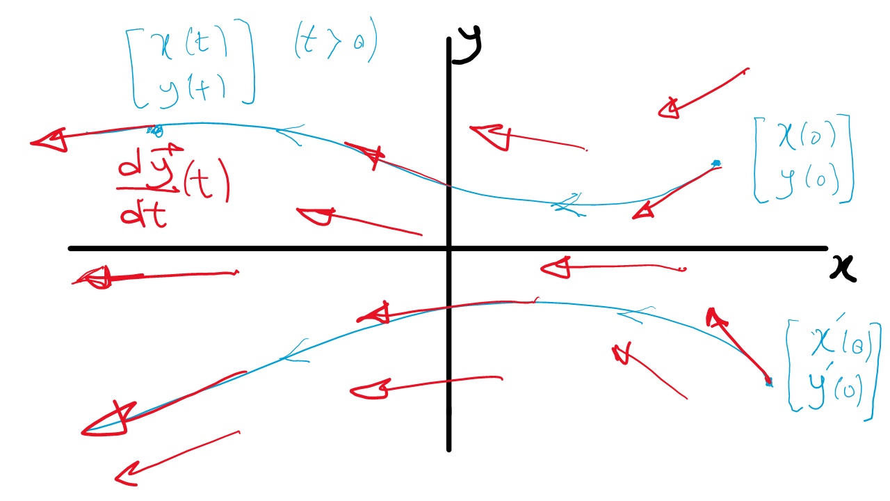
Figure 7.1: Illustration of phase plane for a 2 dimensional system. Two solutions starting at different initial conditions are shown (blue). Also, some representative velocity vectors from the vector field are drawn (red).

One can interpret the phase plane in terms of dynamics. The solution \(\vec{y}(t)\) corresponds to a trajectory of a point moving on the phase plane with velocity \(\dfrac{d\vec{y}}{dt}(t)\). For a system of first order ODEs of the form: \[\dfrac{d\vec{y}}{dt} = F(\vec{y}),\] where, there is no explicit dependence on the independent variable (time) on the right hand side, the velocity is a vector defined at every point of the phase plane and is tangent to the trajectory. This is called the vector field. See Figure 7.1.

Uniqueness of solutions of ODEs

Solutions of ODEs are uniquely defined by initial conditions except at some special points in the phase plane (no proof now, you will see in the second year rigorous proof). Trajectories in the phase plane cannot cross (except at some special points) as this would be equivalent of non-uniqueness of solutions. The special points are fixed points or singular points where trajectories start or end.

Phase plane analysis for the linear systems of first order ODEs

For linear systems, the vector field has some very nice properties. \[\dfrac{d\vec{y}}{dt} = A\vec{y}\] Eigenvectors define very special directions in the phase plane (\(A \vec{v}_1 = \lambda_1 \vec{v}_1\)) in a linear system. The line defined by \(\vec{v}_1\) in the phase plane is an invariant, meaning that if we start on \(\vec{v}_1\), we will remain on it. Let \(\vec{y}(0) = \alpha \vec{v}_1\) with \(\alpha \in \mathbb{R}\). We have: \[A\vec{y}(0) = \alpha A\vec{v}_1 = \alpha \lambda_1 \vec{v}_1 = \frac{d\vec{y}(0)}{dt},\] so, if \(\lambda_1 >0\), \(y(t)\) grows along \(\vec{v}_1\) and if \(\lambda_1 <0\), \(y(t)\) decays along \(\vec{v}_1\) to \(\begin{bmatrix} 0\\ 0 \end{bmatrix}\).

To check this explicitly, we go back to the general solution of systems of ODE (2 dimensional case): \[\vec{y}(t) = c_1 e^{\lambda_1 t} \vec{v}_1 + c_2 e^{\lambda_2 t} \vec{v_2}\]

Let \(\vec{y}(0) = \alpha \vec{v}_1\), this gives \(c_1 = \alpha\) and \(c_2 = 0\). So we have: \[\vec{y}(t) = \alpha e^{\lambda_1 t} \vec{v}_1 = e^{\lambda_1 t} \vec{y}(0),\] so, we see explicitly, from this solution that, if \(\lambda_1 >0\), \(y(t)\) grows along \(\vec{v}_1\) and if \(\lambda_1 <0\), \(y(t)\) decays along \(\vec{v}_1\) to \(\begin{bmatrix} 0\\ 0 \end{bmatrix}\). \(\begin{bmatrix} 0\\ 0 \end{bmatrix}\) is the fixed point of the system as we have \[\frac{d\vec{y}}{dt}\left(\begin{bmatrix} 0\\ 0 \end{bmatrix}\right) = A\begin{bmatrix} 0\\ 0 \end{bmatrix} = \begin{bmatrix} 0\\ 0 \end{bmatrix}. \]

Example 7.4 (First example of qualitative and phase plane analysis of linear systems of ODE) \[\dfrac{d\vec{y}}{dt} = A\vec{y}; \quad A = \begin{bmatrix} -4 & -3 \\ 2 & 3 \end{bmatrix}.\]

We have the solution for this system of linear ODEs using the eigenvalues and eigenvectors for the matrix \(A\):

\[\vec{y}_{GS}(t) = c_1 e^{2 t} \begin{bmatrix} 1\\ -2 \end{bmatrix} + c_2 e^{-3 t} \begin{bmatrix} 3\\ -1 \end{bmatrix}.\]

Next we can look at the asymptotic behavior. Asymptotically, solutions blow up parallel to \(\vec{v}_1\), unless we start on \(\vec{v}_2\), which then we approach \(\vec{y}^* = \begin{bmatrix} 0 \\ 0 \end{bmatrix}\). This is evident from the solution above as if \(c_1 \ne 0\) as \(t \rightarrow \infty\) then \(\vec{y}_{GS} \rightarrow \infty\).

Aim of phase plane analysis is to obtain the phase portrait of the system, which is a summary of all distinct solutions, with qualitatively different trajectories in the phase plane. To do this for our linear system we draw the lines corresponding to the directions of the eigenvectors and trajectories that start on these lines. We consider the asymptotic behavior and we also compute (some examples of the) vector field at some points to draw some representative trajectories. For example, we have at \(\vec{y} = \begin{bmatrix} 1 \\ 0 \end{bmatrix}\): \[ \frac{d\vec{y}}{dt}\left(\begin{bmatrix} 1\\ 0 \end{bmatrix}\right) = A\begin{bmatrix} 1\\ 0 \end{bmatrix} = \begin{bmatrix} -4\\ 2 \end{bmatrix}. \] Figure 7.2 shows the phase portrait for this system. We can explicitly obtain the equations for the trajectories using either the general solution (as seen in the quiz in the lectures) or by obtaining an ODE for \(y(x)\) by dividing the equation for \(\frac{dy}{dt}\) by \(\frac{dx}{dt}\): \[\begin{array}{rl} \dfrac{dx}{dt} = & -4x - 3y \\ \dfrac{dy}{dt} = & 2x + 3y \end{array} \quad \Longrightarrow \quad \dfrac{dy}{dx} = \dfrac{ 2x + 3y}{-4x - 3y} \] This is a homogeneous first order ODE and by using the change of variable \(u = y/x\), we can obtain the following solution. \[(x + 3y)^3(2x + y)^2 = c,\] where \(c\) is a constant of integration and its different values gives us the different trajectories in the phase plane as illustrated in the phase portrait in Figure 7.2. This figure and all the figures in the next section are plotted using the following online applet.

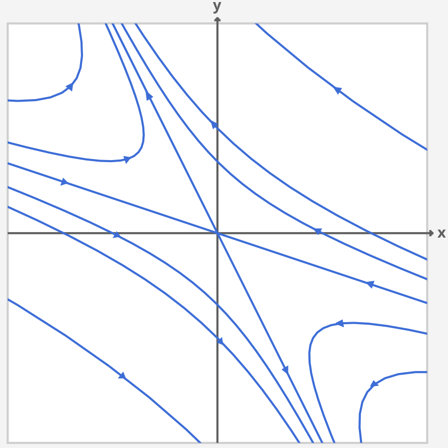
Figure 7.2: The phase portrait for the linear ODE in Example 7.4.

7.3 General system of linear ODEs in 2 dimension

In this section we present a catalogue of qualitative analysis of the general 2 dimensional system of linear ODEs: \[\dfrac{d\vec{y}}{dt} = A \vec{y}; \quad A = \begin{bmatrix} a & b \\ c & d \end{bmatrix}.\] The general solution of this system can be written in terms of the eigenvalues and eigenvectors of matrix \(A\) as seen in the last chapter. The eigenvalues can be obtained by solving the following characteristic equation: \[\lambda^2 - \tau\lambda + \Delta = 0,\] where \(\tau = a + d\) is the trace and \(\Delta = ad - bc\) is the determinant of the matrix \(A\). \[\tau = \text{trace}(A); \quad \Delta = \text{Det}(A); \quad \lambda_1, \lambda_2 = \dfrac{\tau \pm \sqrt{\tau^2 - 4\Delta}}{2}\] The general solution is \[y_{GS} = c_1 e^{\lambda_1 t} \vec{v}_1 + c_2 e^{\lambda_2 t}\vec{v}_2,\] where \(\vec{v}_i\) is the eigenvector corresponding to eigenvalue \(\lambda_i\). In the following we consider the qualitative behaviours of this system for different values in the \((\tau, \Delta)\) plane.

1. Saddle-point or Hyperbolic profile. \(\Delta < 0\); Lower half of \((\tau, \Delta).\)

In this case we have \(\lambda_1 \in \mathbb{R^+}\) and \(\lambda_2 \in \mathbb{R}^-\) since: \[ \Delta < 0 \quad \Longrightarrow \quad \tau^2 - 4\Delta > \tau^2 > 0 \] This is the case similar to Example 7.4 and we have asymptotically as \(t \rightarrow \infty\), \(\vec{y}(t) \rightarrow c_1 e^{\lambda_1}\vec{v_1}\), which grows exponentially as \(\lambda_1\) is a real positive number. However, if we start on the line characterised by \(\vec{v}_2\) direction (i.e. \(c_1 = 0\)), the solution goes to zero. \[ t \rightarrow \infty \quad \Longrightarrow \quad \vec{y} \rightarrow \begin{bmatrix} 0\\ 0 \end{bmatrix}.\] An example of saddle point phase portrait can be seen in Figure 7.3.

Figure 7.3: The saddle point phase portrait. This figure is plotted using this online applet

2.1.1: Repelling or unstable node. \(0<\Delta<\frac{\tau^2}{4}; \, \tau>0.\)

In this case we have \(\lambda_1, \lambda_2 \in \mathbb{R}^+\) and \(\lambda_1>\lambda_2>0\). So starting on \(\vec{v}_2\) blow-up along the direction of \(\vec{v}_2\). Otherwise, blow up in the direction of \(\vec{v}_1\). \[t \rightarrow \infty \quad \Longrightarrow \quad \vec{y}(t) \rightarrow c_1 e^{\lambda_1}\vec{v_1} \rightarrow \infty.\]

An example of repelling or unstable node phase portrait can be seen in Figure 7.4.

Figure 7.4: The repelling or unstable node phase portrait. This figure is plotted using this online applet

2.1.2: Attracting or stable node. \(0<\Delta<\frac{\tau^2}{4}; \tau<0.\)

In this case we have \(\lambda_1, \lambda_2 \in \mathbb{R}^-\) and \(\lambda_2<\lambda_1<0\). So starting on \(\vec{v}_2\) decays to \(\begin{bmatrix} 0 \\ 0 \end{bmatrix}\) along the direction of \(\vec{v}_2\). Otherwise, decays along the direction of \(\vec{v}_1\) to \(\begin{bmatrix} 0 \\ 0 \end{bmatrix}\). So, for \(c_1 \ne 0\), we have: \[t \rightarrow \infty \quad \Longrightarrow \quad \vec{y}(t) \rightarrow c_1 e^{-|\lambda_1|}\vec{v_1} \rightarrow \begin{bmatrix} 0 \\ 0 \end{bmatrix}.\] An example of attracting or stable node phase portrait can be seen in Figure 7.5.

Figure 7.5: The attracting or stable node phase portrait. This figure is plotted using this online applet

2.2.1: Centre or elliptic profile. \(\Delta>\frac{\tau^2}{4}; \, \tau=0\)

In this case \(\lambda_{1,2} = \pm i \omega\) and the solution is periodic. Periodic behaviour corresponds to closed curves in the phase plane. For linear systems the closed curves are ellipses.

Example 7.5 (Harmonic oscillator: revisited) \[\frac{x^2}{dt^2} + \omega^2 x = 0.\]

We can write this second order linear ODE as a system of two first order linear ODEs, but defining \(y = \frac{dx}{dt}\). The general solution for this system can be written as: \[\begin{bmatrix} x_{GS} \\ y_{GS} \end{bmatrix} = \begin{bmatrix} A_0 \sin(\omega t + \phi) \\ A_0 \omega \cos(\omega t + \phi) \end{bmatrix}.\] From this result we see that the trajectory of solutions are ellipses. \[x^2 + \frac{y^2}{\omega^2} = A_0^2 = x_0^2 + \frac{y_0^2}{\omega^2},\] where \(A_0\) is a constant of integration and it depends on the initial conditions \(x_0\) and \(y_0\).

The phase portrait illustrating the elliptic profile can be seen in Figure 7.6. To figure out the direction of motion we evaluate the vector field at some points: \[\vec{y} = \begin{bmatrix} 0 \\ y \end{bmatrix} \quad \Rightarrow \quad \frac{d\vec{y}}{dt} = A \vec{y} = \begin{bmatrix} y \\ 0 \end{bmatrix},\]

\[\vec{y} = \begin{bmatrix} x \\ 0 \end{bmatrix} \quad \Rightarrow \quad \frac{d\vec{y}}{dt} = A \vec{y} = \begin{bmatrix} 0 \\ -\omega^2 x \end{bmatrix}.\]

Note that in this case the point \(\vec{y} = \begin{bmatrix} 0 \\ 0 \end{bmatrix}\) is a stable fixed point, with Lyapunov stability as the trajectories around the origin do not blow up but also do not asymptotically approach the origin.

Figure 7.6: The centre or elliptic phase portrait. This figure is plotted using this online applet

2.2.2: Repelling or unstable spiral. \(\Delta>\frac{\tau^2}{4}; \, \tau>0.\)

The eigenvalues are complex with the real part being postive. So, for the general solution we have: \[\vec{y} = e^{\frac{\tau}{2}t} \left[c_1 e^{i\omega t} \vec{v}_1 + c_2 e^{-i\omega t} \vec{v}_2 \right], \] which, asymptotically blow up in an oscilatory fashion. The phase portrait illustrating the repelling or unstable spiral can be seen in Figure 7.7.

Figure 7.7: The repelling or unstable spiral phase portrait. This figure is plotted using this online applet

2.2.3: Attracting or stable spiral. \(\Delta>\frac{\tau^2}{4}; \, \tau<0\)

The eigenvalues are complex with the real part being negative. So, for the general solution we have:
\[\vec{y} = e^{\frac{\tau}{2}t} \left[c_1 e^{i\omega t} \vec{v}_1 + c_2 e^{-i\omega t} \vec{v}_2 \right],\] which, asymptotically as \(t \rightarrow \infty\), \(\vec{y} \rightarrow \begin{bmatrix} 0 \\ 0 \end{bmatrix}\). The phase portrait illustrating the attracting or stable spiral can be seen in Figure 7.8.

Figure 7.8: The attracting or stable spiral phase portrait. This figure is plotted using this online applet

3.1: Line of repelling or unstable fixed points. \(\Delta = 0; \quad \tau>0\).

In this case we have \(\lambda_1 = \tau\) and \(\lambda_2 = 0\), so the general solution is: \[\vec{y} = c_1 e^{\tau t} \vec{v}_1 + c_2 \vec{v}_2.\] For the vector field we have: \[\dfrac{d\vec{y}}{dt} = c_1 \tau e^{\tau t}\vec{v}_1,\] So, \(y^* = c_2 \vec{v}_2\) is a line of unstable fixed points. Asymptotically as \(t \rightarrow \infty\) then \(\vec{y}(t) \rightarrow c_1 \tau e^{\tau t}\vec{v}_1\), which blows up exponentially in the direction of \(\vec{v}_1\). The phase portrait for this case can be seen in Figure 7.9.

Figure 7.9: Line of repelling or unstable fixed points phase portrait. This figure is plotted using this online applet

3.2: Line of attracting or stable fixed points. \(\Delta = 0; \quad \tau<0.\)

In this case we have \(\lambda_1 = \tau\) and \(\lambda_2 = 0\) again similar to last case and the general solution is \[\vec{y} = c_1 e^{\tau t} \vec{v}_1 + c_2 \vec{v}_2.\] For the vector field we have: \[\dfrac{d\vec{y}}{dt} = c_1 \tau e^{\tau t}\vec{v}_1.\] So, \(y^* = c_2 \vec{v}_2\) is a line of stable fixed points. Asymptotically as \(t \rightarrow \infty\) then \(\vec{y}(t) \rightarrow c_1 \tau e^{\tau t}\vec{v}_1\), which decays exponentially to the line of \(c_2\vec{v}_2\). The phase portrait for this case can be seen in Figure 7.10.

Figure 7.10: line of attracting or stable fixed points phase portrait. This figure is plotted using this online applet

4.1: Repelling (4.1.1) and attracting (4.1.2) star node. \(\tau^2 - 4\Delta = 0\)

In this case the eigenvalues are repeated \(\lambda_1 = \lambda_2 = \frac{\tau}{2}\) and \(A\) is diagonalizable. We have: \[A = \begin{bmatrix} \lambda & 0\\ 0 & \lambda \end{bmatrix} \quad \Rightarrow \quad \vec{v}_1 = \begin{bmatrix} 1\\ 0 \end{bmatrix}, \quad \vec{v}_2 = \begin{bmatrix} 0\\ 1 \end{bmatrix}.\] So, we have for the general solution \[\vec{y} = c_1 e^{\lambda t} \begin{bmatrix} 1\\ 0 \end{bmatrix} + c_2 e^{\lambda t} \begin{bmatrix} 0\\ 1 \end{bmatrix} = e^{\lambda t} \begin{bmatrix} c_1\\ c_2 \end{bmatrix}.\]

We observe that in this case, the trajectory is always defined by \(\vec{y}(0)\). The phase portrait for the repelling star node (4.1.1) can be seen in Figure 7.11. The attracting star node phase portrait is similar with an asymptotically stable fixed point at the origin \(\begin{bmatrix} 0\\ 0 \end{bmatrix}\).

Figure 7.11: Repelling star node phase portrait. This figure is plotted using this online applet

4.2: Unstable (4.2.1) and stable (4.2.2) improper or degenerate node. \(\tau^2 - 4\Delta = 0\)

In this case the eigenvalues are repeated \(\lambda_1 = \lambda_2 = \frac{\tau}{2}\) but \(A\) is non-diagonalizable and \(\tau > 0\) (unstable 4.2.1) or \(\tau <0\) (stable 4.2.2).

Example 7.6 \[\dfrac{d\vec{y}}{dt} = A \vec{y}; \quad A = \begin{bmatrix} 1 & -1 \\ 1 & 3 \end{bmatrix}.\]

In this last chapter, using the Jordan normal form, we showed the general solution of this system of ODEs to be: \[\vec{y}_{GS} = (c_1e^{2t} + c_2 t e^{2t})\vec{v}_1 + c_2 e^{2t}\vec{w}_2,\] where \(\vec{v}_1 = \begin{bmatrix} 1 \\ -1 \end{bmatrix}\) is the only eigenvector, and \(\vec{w}_2 = \begin{bmatrix} 1 \\ -2 \end{bmatrix}\). We see that as \(t \rightarrow \infty\), \(\vec{y}(t)\) blows up in the direction of \(\vec{v}_1\). We can estimate the vector field at specific points to helps draw the phase portrait. The phase portrait for this case can be seen in Figure 7.12, which is of the type unstable improper or degenerate node (4.2.1). Stable improper or degenerate node (4.2.2) have a similar phase portrait to this with an asymptotically stable fixed point at the origin \(\begin{bmatrix} 0\\ 0 \end{bmatrix}\).

Figure 7.12: Unstable improper or degenerate node phase portrait. This figure is plotted using this online applet

The catalogue of phase portraits for the 2 dimensional linear systems of ODEs can be seen in Figure 7.13 on the \((\tau, \Delta)\) plane. We note that the solutions can be unstable, asymptotically stable or Lyapunov stable in the different regions of \((\tau, \Delta)\) plane. The system can have one fixed point or infinitely many fixed points. Also, solutions could be oscillatory or non-oscillatory in different regions of the parameter space.

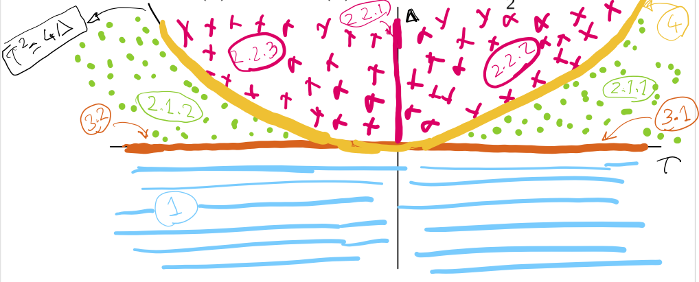
Figure 7.13: The catalogue of phase portraits for the 2 dimensional linear systems of ODEs

7.4 Phase plane analysis for 2D nonlinear systems

Phase plane analysis is a very useful tool for 2 dimensional nonlinear systems and the insights obtained from the 2D linear case is highly relevant. One obtains the special points (fixed points) and could linearise the equations in the vicinity of these points to get insight from the analysis of the corresponding linear system. Vector field and asymptotic behaviour is useful to identify the trajectories in the phase plane.

Example 7.7 (Synthetic Biology: Genetic Toggle Switch)

This model of a simple synthetic genetic network was proposed in a pioneering paper by Gardener, Cantor and Colins, Nature 403:339-342 (2000). Consider two genes \(u\) and \(v\), which inhibit expression of one another. The following system of nonlinear ODEs characterises the dynamics between the two genes.
\[\begin{align*} \frac{du}{dt} &= \frac{\alpha_1}{1 + v^\beta} - u,\\ \frac{dv}{dt} &= \frac{\alpha_2}{1 + u^\gamma} - v. \end{align*}\] Characterising the fixed points of this model, allowed the authors to successfully design and construct one of the first synthetic genetic networks. This system has up to 3 fixed points (two stable and one unstable ones).

Example 7.8 (Lotka-Voltera Model)

Consider this classic model of predator-prey, where \(x>0\) denotes number of rabbits and \(y>0\) number of foxes in a population (with \(a, b, c, d>0\)). \[\begin{align*} \frac{dx}{dt} &= ax - bxy,\\ \frac{dy}{dt} &= dxy - cy. \end{align*}\] By setting the derivatives to zero, we obtain the following two fixed points for the system. \[\begin{bmatrix} x^* \\ y^* \end{bmatrix}_1 = \begin{bmatrix} 0 \\ 0 \end{bmatrix}, \quad \begin{bmatrix} x^* \\ y^* \end{bmatrix}_2 = \begin{bmatrix} c/d \\ a/b \end{bmatrix}.\] We consider dynamics near each fixed points by considering \[x = x^* + \Delta x,\] \[y = y^* + \Delta y,\] where, \(\Delta x, \Delta y << 1\). Linearising around the first fixed point by omitting terms of the order of \(\Delta x \Delta y\), we obtain: \[\begin{align*} \frac{d\Delta x}{dt} &= a\Delta x ,\\ \frac{d\Delta y}{dt} &= -c\Delta y. \end{align*}\] This is a 2D linear system of ODEs that exhibits a saddle-point phase portrait suggesting that the first fixed point is unstable. Similarly, linearising around the second fixed point, we obtain: \[\begin{align*} \frac{d\Delta x}{dt} &= -\frac{bc}{d} \Delta y ,\\ \frac{d\Delta y}{dt} &= \frac{da}{b}\Delta x. \end{align*}\] This is a 2D linear system of ODEs that exhibits a centre phase portrait suggesting that the second fixed point has Lyapunove stability. Putting these together we get the phase portrait in Figure 7.14 for the Lotka-Voltera Model that suggests the system has periodic trajectories around the second fixed point in the phase plane.

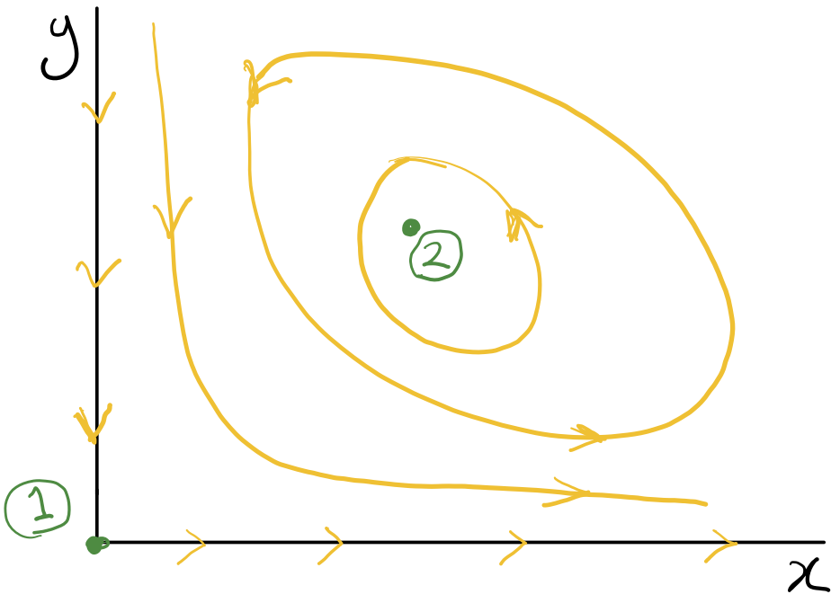
Figure 7.14: The phase portraits for the Lotka-Voltera model

7.5 Extension of phase plane analysis to higher dimensional systems

1. \(\vec{y}(t)\) can be considered a trajectory in \(\mathbb{R}^n\), where \(n\) is the dimensionality of the system.
2. From each initial condition there is a unique trajectory and trajectories do not cross except at some special points.
3. We can consider asymptotic behavior to draw the trajectories.
4. We can compute vector field: \[\frac{d\vec{y}}{dt} = \vec{F}(\vec{y}).\]
5. Fixed points (\(\vec{y}^*\)) are obtained by: \[\frac{d\vec{y}}{dt}\left(\vec{y}^*\right) = \vec{0}.\]

The approach directly generalises for the linear systems as the solutions are given by the eigenvectors and eigenvalues of matrix \(A\). As in the 2 dimensional case, solutions starting in the directions set by the eigenvectors, stay on these directions and grow or decay depending on the sign of the corresponding eigenvalue.

Stability of linear \(n\) dimensional systems For the 2 dimensional case we had stability where \(\tau \le 0\) and \(\Delta \ge 0\). In terms of eigenvalue characterization this meant the real part of the eigen values are negative. Similarly, for the general \(n\) dimensional linear systems of ODEs we have stability if the real part of all the eigenvalues are negative.

Lorenz system (1933, Edward Lorenz)

More complex dynamics in phase planes are possible. Lorenz proposed a system of 3 nonlinear equations that is a model of atmospheric convection. This rather simple model for certain values of parameters (e.g. \(\sigma = 10\), \(\beta = \frac{8}{3}\) and \(\rho = 28\)), exhibits a complex non-periodic dynamics that is an example of chaos. This dynamical behavior is characterised by the divergence of trajectories in the phase plane starting from near identical initial conditions as illustrated in this video. \[\begin{align*} \frac{dx}{dt} &= \sigma (y -x),\\ \frac{dy}{dt} & = x(\rho - z) - y,\\ \frac{dz}{dt} & = xy - \beta z. \end{align*}\]