Chapter 8 Introduction to Bifurcations

Bifurcations in a dynamical system (system of ODEs) describe the qualitative change in behavior under a variation or change of some parameters of the system. Parameters are constants that are tunable.

8.1 Bifurcations in linear systems

We start by looking at linear systems, first through an example:

Example 8.1 (Taking $k$ to be the tuning parameter in the damped harmonic oscilator system) \[\dfrac{d^2x}{dt^2} + 2k \dfrac{dx}{dt} + \omega^2 x = 0\]

How does the qualitative behavior of $x(t; k)$ change when $k \in \mathbb{R}$ is varied?

We know this system is equivalent to a system of linear first order linear ODEs, letting $u = \frac{dx}{dt}$ we have: \[\frac{d}{dt}\begin{bmatrix} x \\ u \end{bmatrix} = \begin{bmatrix} 0 & 1 \\ -\omega^2 & - 2k \end{bmatrix} \begin{bmatrix} x \\ u \end{bmatrix}.\] Given the catalogue of phase portraits in the $(\tau, \Delta)$ plane we saw in the last chapter, we can use these to see how the qualitative behavior of $\vec{y}(t; k) = \begin{bmatrix} x \\ u \end{bmatrix}$ changes when $k$ is varied. For this system we have $\tau = -2k$ and $\Delta = \omega^2$, so only $\tau$ depends on the tunable parameter $k$ and $\Delta$ is always positive. As Figure 8.1 shows there are 7 different phase portraits that can be observed as $k$ is varied. Defining a bifurcation as a change in stability of the system, there is only one bifurcation point at $k = 0$ for this system.

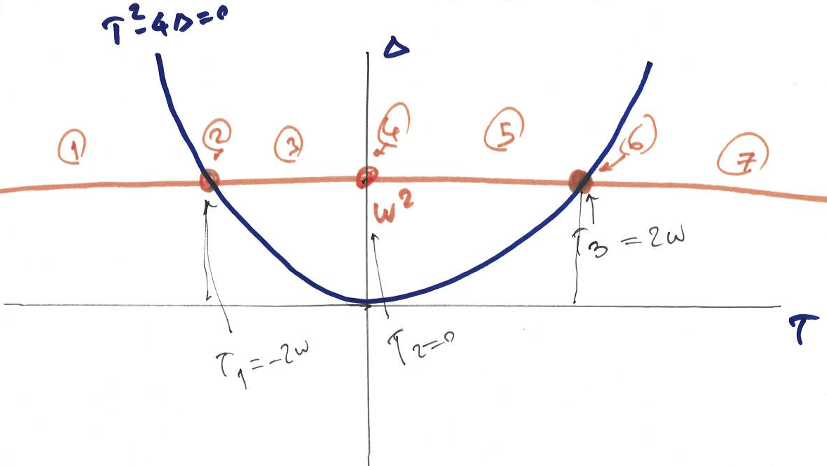
Figure 8.1: Qualitative behavior of the damped harmonic oscillator system as $k$ is varied

In linear systems the bifurcations are related to changes in the stability of the system, as that is the main type of change that can happen in the dynamics of the system.

In non-linear systems there is a whole zoo of bifurcations and we will not cover these here but we will consider one dimensional nonlinear systems in the next section.

8.2 Qualitative behavior of non-linear 1D systems

Consider the general one dimensional nonlinear first order ODE. \[\dfrac{dy}{dt} = f(y); \quad y \in \mathbb{R}^1\]

The phase plane for 1D systems can be considered. We have:

$y(t)$ are trajectories on the real line.
Vector field describing how we move is the velocity and is scalar in 1D case ($f(y) \in \mathbb{R}$).
special points include
1. Fixed points: $f(y^*) = 0$.
2. Singularities where $f(y_{sing})$ is non-defined.

Example 8.2 (First (trivial) example of the phase plane and bifurcation analysis in one dimension) \[\dfrac{dy}{dt} = ky = f(y; k).\]

The fixed point for this system is $y^* = 0$ as $f(y*=0) = 0$. The general solutio for this ODE is \[y(t; k) = y(0)e^{kt}.\] The general solution suggests that the fixed point is stable for $k<0$ and is unstable for $k>0$. Also, we can also use a plot of $\dfrac{dy}{dt} = f(y; k)$ vs $y$ for different values of $k$ to draw the vector field as illustrated in Figure 8.2 to obtain the stability of the fixed points. A stable fixed point has a flow towards it, while an unstable fixed points has an outward flow.

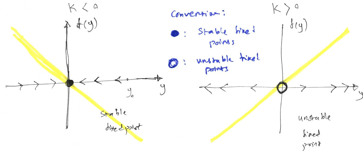
Figure 8.2: The plot of $f(y)$ vs $y$ for different values of $k$, illustrates the vector field and the stability of the fixed point for Example 8.2.

A bifurcation diagram summarises all possible behaviours of the system as a parameter is varied. It represents all fixed points of the system and their stability as a function of the varying parameter. The bifurcation diagram for this example is drawn in Figure 8.3.

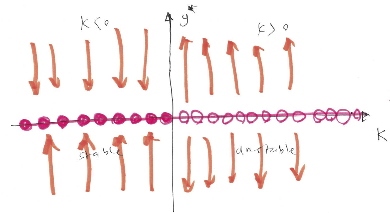
Figure 8.3: The bifurcation diagram (plot of fixed points and their stability vs the tuning parameter $k$) for Example 8.2.

There are only 3 kinds of nonlinear 1D systems in terms of their bifurcation.

8.2.1 Saddle-node bifurcation

This is a basic mechanism for creation and destroying fixed points. The prototypical example of saddle-node bifurcation is given by: \[\dfrac{dy}{dt} = r + y^2,\] where $r \in \mathbb{R}$. We have $y^* = \pm\sqrt{-r}$. Figure 8.4 using the vector field, illustrates number and stability of these fixed points for different values of $r$.

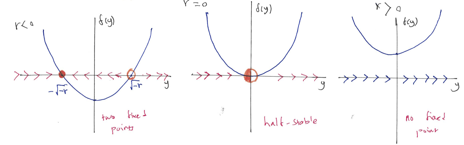
The plot of $f(y)$ vs $y$ for different values of $r$, illustrates the vector field and the stability of the fixed point for saddle-node bifurcation.

Figure 8.4: The plot of $f(y)$ vs $y$ for different values of $r$, illustrates the vector field and the stability of the fixed point for saddle-node bifurcation.

For $r<0$ we have 2 fixed points (one stable, one unstable), at $r=0$ we have one half-stable fixed point and for $r>0$ we have no fixed point. There is a saddle-node bifurcation at $r=0$. These changes in the number and stability of the fixed points can be summarised using the bifurcation diagram, which is a plot of fixed points vs parameter $r$ (see Figure 8.5).

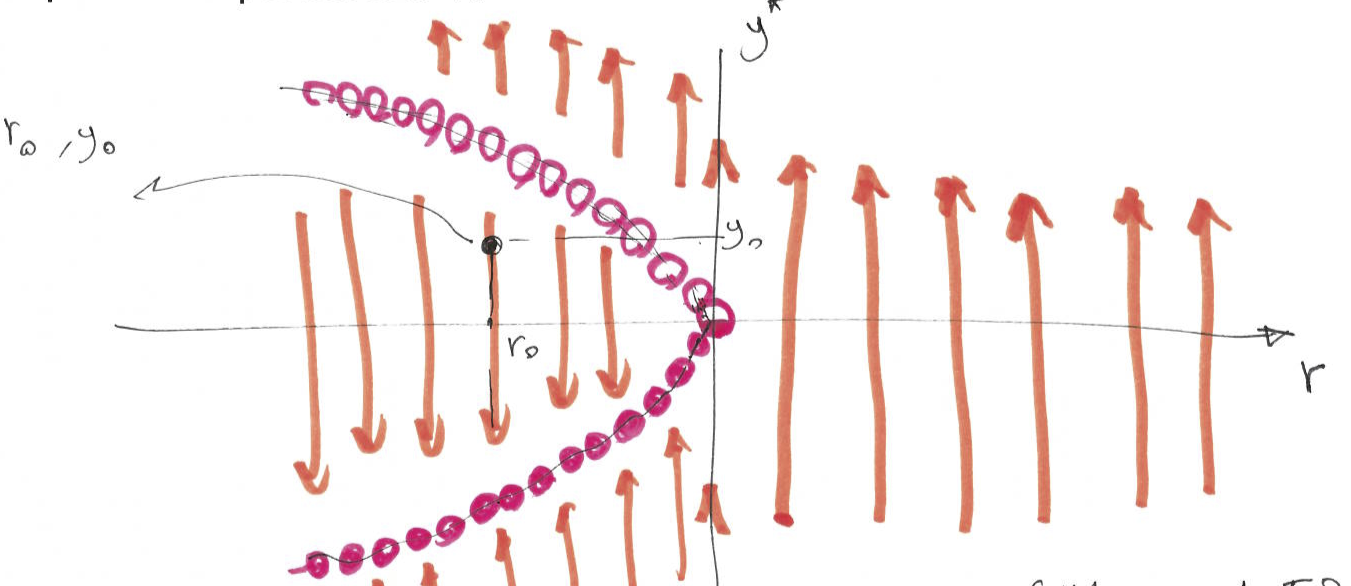
Figure 8.5: The bifurcation diagram (plot of fixed points and their stability vs the tuning parameter $r$) for saddle-node bifurcation.

8.2.2 Transcritical bifurcation

In certain systems a fixed point must exist for all values of a parameter. The prototypical example of this form of bifurcation is given by: \[\dfrac{dy}{dt} = ry - y^2,\] where $r \in \mathbb{R}$. This ODE has up to two fixed points $y^* = 0$ and $y^* = r$. Figure 8.6 using the vector field, illustrates number and stability of these fixed points for different values of $r$.

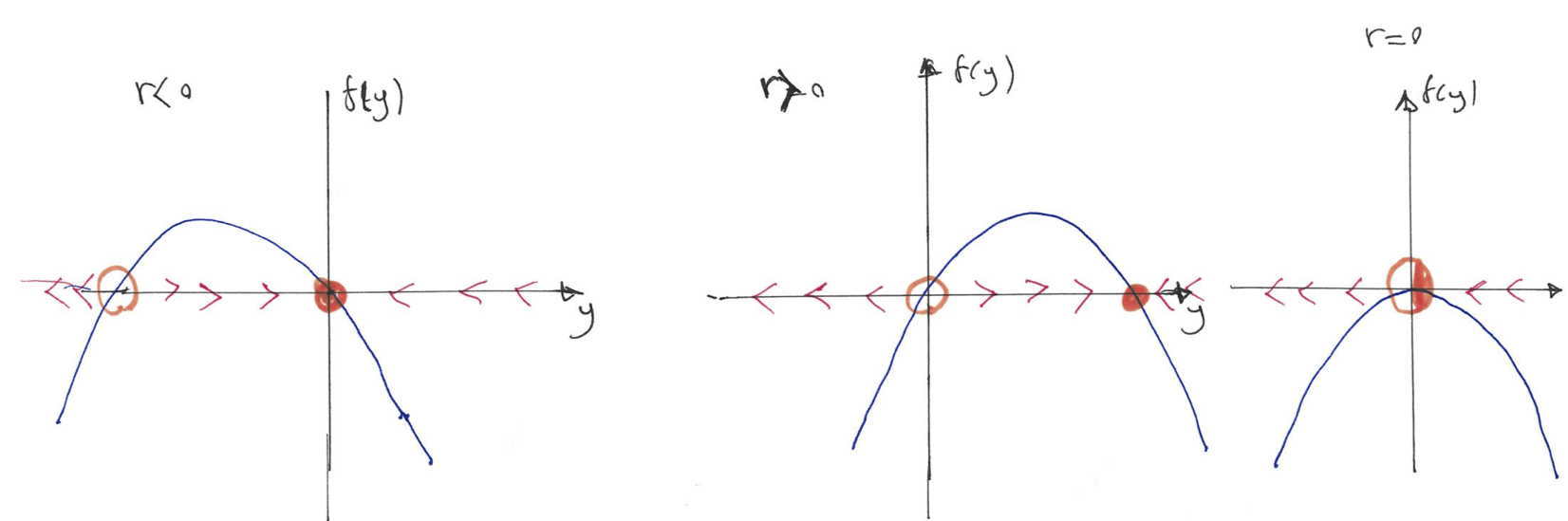
The plot of $f(y)$ vs $y$ for different values of $r$, illustrates the vector field and the stability of the fixed point for transcritical bifurcation.

Figure 8.6: The plot of $f(y)$ vs $y$ for different values of $r$, illustrates the vector field and the stability of the fixed point for transcritical bifurcation.

For $r<0$ we have 2 fixed points (one stable, one unstable), at $r=0$ we have one half-stable fixed point and for $r>0$ go back to two fixed points. At the bifurcation point $r=0$ an exchange of stabilities takes place between the two fixed points. The changes in the number and stability of the fixed points is summarised in the bifurcation diagram (see Figure 8.7).

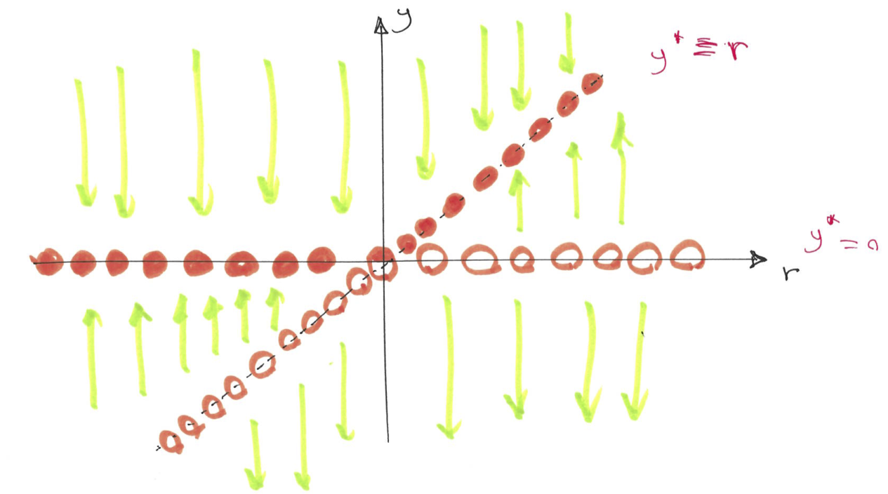
Figure 8.7: The bifurcation diagram (plot of fixed points and their stability vs the tuning parameter $r$) for transcritical bifurcation.

8.2.3 Pitchfork bifurcation

This kind of bifurcation is common in physical systems that have a symmetry. There are two subtypes of pitchfork bifurcation.

Supercritical pitchfork bifurcation

The prototypical example of supercritical pitchfork bifurcation is given by: \[\dfrac{dy}{dt} = ry- y^3 = f(y; r)\]

Note that the equation is invariant under the change of variable $y \rightarrow -y$, which signifies the symmetry. The system has up to three fixed points $y^* = 0$ and $y^* = \pm \sqrt{r}$. Figure 8.8 using the vector field, illustrates number and stability of these fixed points for different values of $r$.

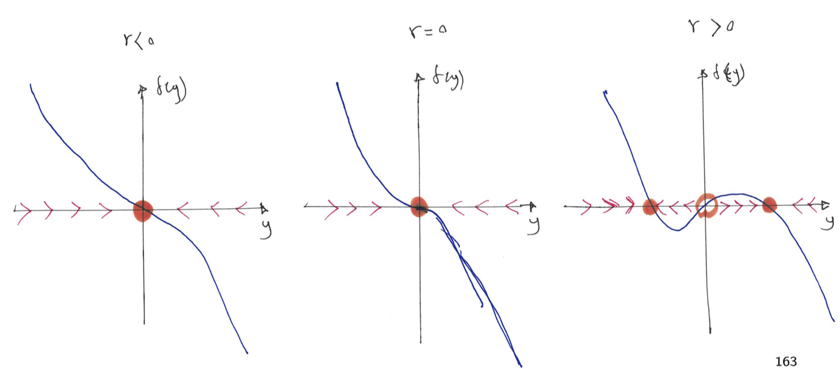
The plot of $f(y)$ vs $y$ for different values of $r$, illustrates the vector field and the stability of the fixed point for supercritical pitchforkbifurcation.

Figure 8.8: The plot of $f(y)$ vs $y$ for different values of $r$, illustrates the vector field and the stability of the fixed point for supercritical pitchforkbifurcation.

For $r<0$ we have 1 stable fixed point, at $r=0$ we have still one stable fixed point and for $r>0$ we have three fixed points (two stable and a middle one that is unstable). At the bifurcation point $r=0$ an exchange of stabilities takes place between the fixed points. The changes in the number and stability of the fixed points is summarised in the bifurcation diagram (see Figure 8.9).

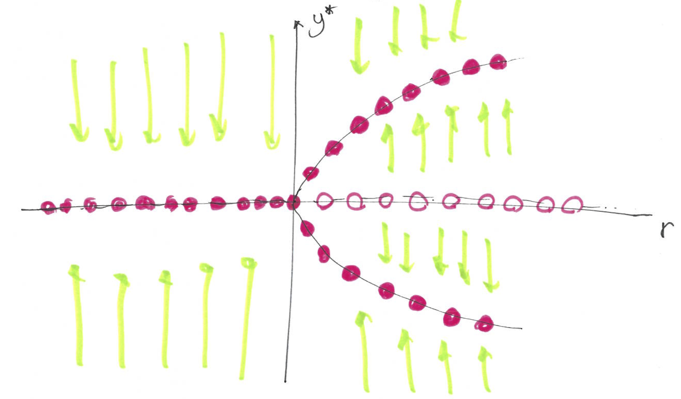
Figure 8.9: The bifurcation diagram (plot of fixed points and their stability vs the tuning parameter $r$) for supercritical pitchfork bifurcation.

Subcritical pitchfork bifurcation

In the subcritical pitchfork bifurcation in contrast to the supercritical case the cubic term is destabilising:

\[\dfrac{dy}{dt} = ry + y^3 = f(y; r)\]

The system again has up to three fixed points $y^* = 0$ and $y^* = \pm \sqrt{-r}$. Figure 8.10 using the vector field, illustrates number and stability of these fixed points for different values of $r$.

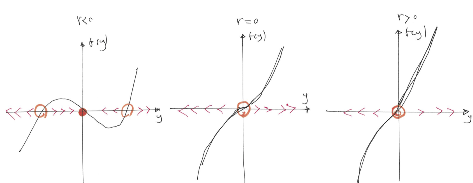
The plot of $f(y)$ vs $y$ for different values of $r$, illustrates the vector field and the stability of the fixed point for subcritical pitchfork bifurcation.

Figure 8.10: The plot of $f(y)$ vs $y$ for different values of $r$, illustrates the vector field and the stability of the fixed point for subcritical pitchfork bifurcation.

For $r<0$ we have we have three fixed points (two unstable and a middle one that is stable), at $r\ge 0$ we have one unstable fixed point. At the bifurcation point $r=0$ an exchange of stabilities takes place between the fixed points. The changes in the number and stability of the fixed points is summarised in the bifurcation diagram (see Figure 8.11).

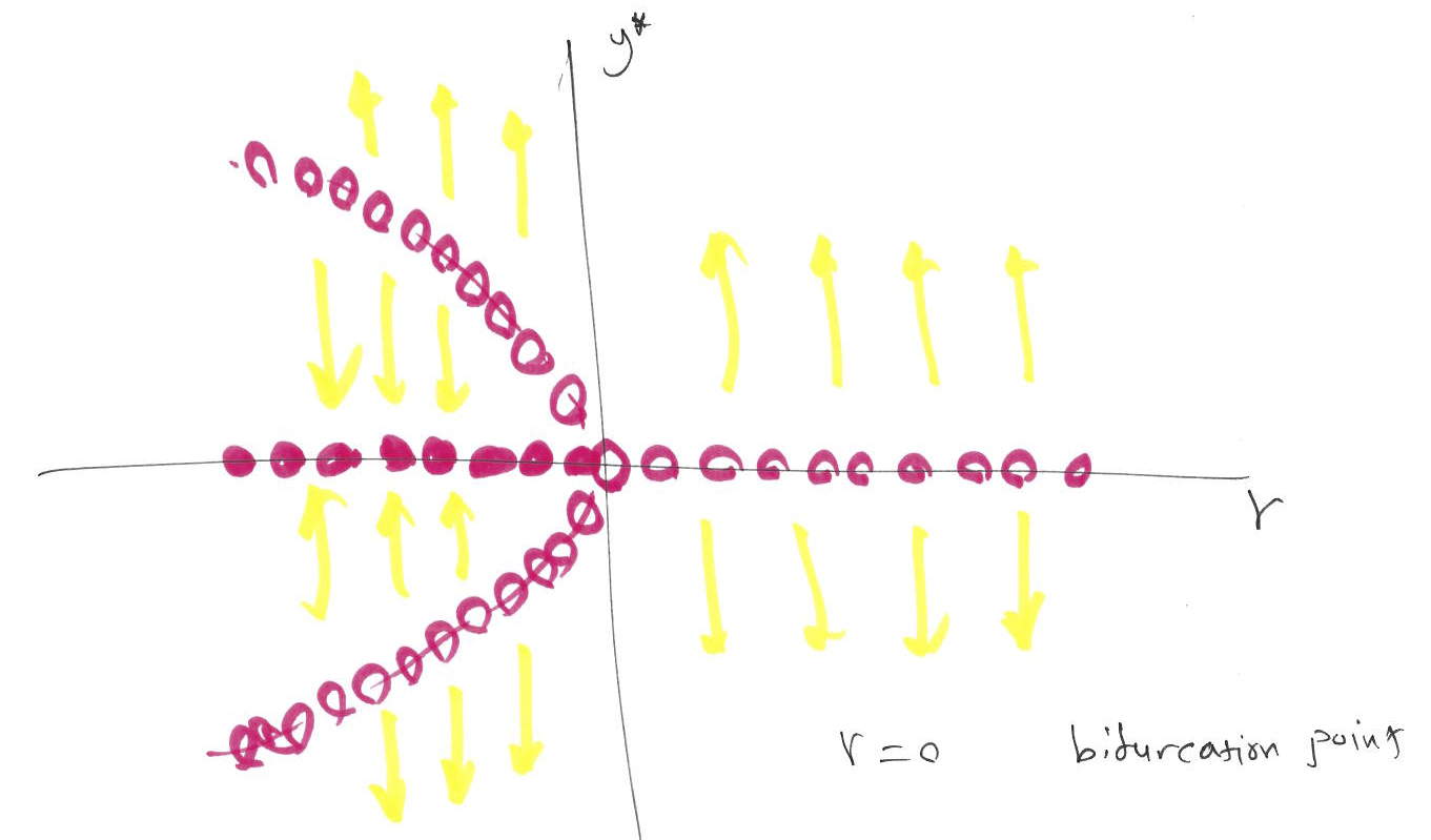
Figure 8.11: The bifurcation diagram (plot of fixed points and their stability vs the tuning parameter $r$) for subcritical pitchfork bifurcation.

8.2.4 Singular points

As at the beginning of this section the special points can be the fixed points $y^*$ or the singularities $y_{sing}$, where the $f(y_{sing}; r)$ is not defined.

Example 8.3 (An example of an ODE with singularity) \[\dfrac{dy}{dt} = \dfrac{k}{y} = f(y, k)\]

Here, $f(y; k)$ is not defined at $y_{sing} = 0$. Figure 8.12 using the vector field, shows the stability of the singularity for different values of $k$.

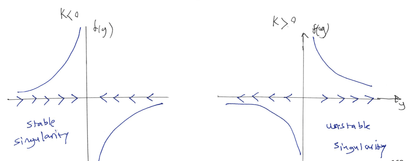
Figure 8.12: The plot of $f(y)$ vs $y$ for different values of $k$, illustrates the vector field and the stability of the singularity in Example 8.3.

For this example, we have an explicit solution that provides further insight in the behavior of the system for different values of $k$ and initial condition.

\[\dfrac{dy}{dt} = \dfrac{k}{y} \quad \Longrightarrow \quad \int ydy = \int k dt \quad \Longrightarrow \quad y = \pm \sqrt{2kt + y_0^2},\] where $y_0 = y(t= 0)$ is the inital condition. For $y_0>0$, we have the positive solution and for $y_0<0$, we have the negative solution. Also, for $k>0$ the solutions blow up to infinity and for $k<0$ solutions approach $0$. This is summarised in the bifurcation diagram (see Figure 8.13).

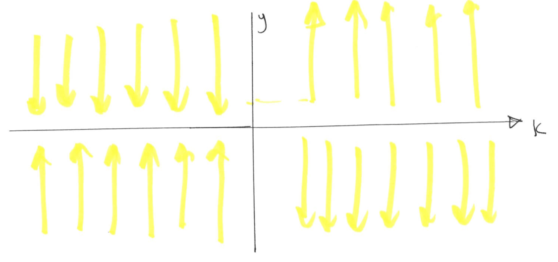
Figure 8.13: The bifurcation diagram (plot of singular points and their stability vs the tuning parameter $k$) for Example 8.3.

8.2.5 Impossibility of oscillations for one dimensional systems

Fixed points dominate the dynamics of first-order systems. The trajectory in one dimension phase plane never reverses direction and the approach to equilibrium is always monotonic, hence there is no over-shoot, damped oscillations or periodic solutions. This is a topological constraint, if you flow monotonically on a line, you’ll never come back to your starting point. Of course, if we were moving on a circle rather than a line, we could eventually return to starting point. For example the following ODE $\frac{d\theta}{dt} = \omega$ for the angle $\theta$ has the following periodic solution $\theta = \omega t + \theta_0$.

8.2.6 Linear stability analysis

So far we have relied on graphical methods to determine stability of fixed points (using the flows of the vector field). A quantitative measure can be obtained by linearizing about the fixed point for the one dimensional systems. Let $\eta = y - y^*$ be a small perturbation away from the fixed point $y^*$. We have using the Taylor expansion of $f(y)$. \[ \frac{dy}{dt} = \frac{d\eta}{dt} = f(y^* + \eta) = f(y^*) + \eta \frac{df}{dy}(y = y^*) + \cdots \quad \Rightarrow \quad \frac{d\eta}{dt} \approx \eta \frac{df}{dy}(y^*).\]

Now, if $\frac{df}{dy}(y^*) > 0$ then the fixed point $y^*$ is unstable as the perturbations around the fixed point grow. However, if $\frac{df}{dy}(y^*) < 0$ then the fixed point $y^*$ is stable as the perturbations around the fixed point decay to zero.