Chapter 2 Properties of Fourier Transforms
In the following we present some important properties of Fourier transforms. These results will be helpful in deriving Fourier and inverse Fourier transform of different functions. After discussing some basic properties, we will discuss, convolution theorem and energy theorem. Finally, we introduc Dirac delta function.
2.1 Basic Properties
- (i) The Fourier and inverse Fourier transforms are linear, and so \[\mathcal{F}\{af(x) + bg(x)\} = a\hat{f}(\omega) + b\hat{g}(\omega),\] \[\mathcal{F}^{-1}\{a\hat{f}(\omega) + b\hat{g}(\omega)\} = af(x) + bg(x),\] where \(a\) and \(b\) are constants and \(\mathcal{F}^{-1}\) denotes the inverse Fourier transform.
-(ii) If \(a>0\):
\[\mathcal{F}\{f(ax)\} = \frac{1}{a}\hat{f}(\frac{\omega}{a}).\] Proof Starting on the LHS, and making the substitution \(s = ax\): \[\mathcal{F}\{f(ax)\} = \int_{-\infty}^{\infty} f(ax)e^{-i\omega x} \,dx = \frac{1}{a} \int_{-\infty}^{\infty} f(s)e^{-i(\omega/a) s} \,ds = \frac{1}{a} \hat{f}(\frac{\omega}{a}).\]
-(iii) In a similar way we can establish that \[\mathcal{F}\{f(-x)\} = \hat{f}(-\omega).\]
-(iv) The transform of a shifted function can be calculated as follows (using \(s = x − x_0)\):
\[\mathcal{F}\{f(x- x_0)\} = \int_{-\infty}^{\infty} f(x- x_0)e^{-i\omega x} \,dx = \int_{-\infty}^{\infty} f(s)e^{-i\omega(s+ x_0)} \,ds = e^{-i\omega x_0} \hat{f}(\omega).\]
-(v) A similar result, but this time involving a shift in transform space:
\[\mathcal{F}\{e^{i\omega_0 x}f(x)\} = \int_{-\infty}^{\infty} f(x)e^{-i(\omega - \omega_0) x} \,dx = \hat{f}(\omega - \omega_0).\]
-(vi) Symmetry formula The following result is very useful. Suppose the Fourier transform of \(f(x)\) is \(\hat{f}(\omega)\); change the variable \(\omega\) to \(x\); then
\[\mathcal{F}\{\hat{f}(x)\} = 2\pi f(-\omega).\] Proof Starting with the inversion formula and changing variables from \(\omega\) to \(s\), we have \[f(x) = \frac{1}{2\pi} \int_{-\infty}^{\infty} \hat{f}(\omega) e^{i\omega x} \, d\omega = \frac{1}{2\pi} \int_{-\infty}^{\infty} \hat{f}(s) e^{i s x} \, ds.\] If we now let \(x = -\omega\) and then \(s = x\), we get: \[f(-\omega) = \frac{1}{2\pi} \int_{-\infty}^{\infty} \hat{f}(s) e^{-i\omega s} \, ds = \frac{1}{2\pi} \int_{-\infty}^{\infty} \hat{f}(x) e^{-i\omega x} \, dx = \frac{1}{2\pi}\ \mathcal{F}\{\hat{f}(x)\},\] as required.
The following results are particularly useful when applying Fourier transforms to differential equations (as seen later this term and next year in the context of partial differential equations).
-(vii)
\[\mathcal{F}\{\frac{d^nf}{dx^n}\} = (i\omega)^n \hat{f}(\omega).\]
Proof This can be established by integration by parts. We assume that all derivatives of \(f\) tend to zero as \(x \rightarrow \pm \infty\).
\[\begin{align*} \mathcal{F}\{d^nf/dx^n\} & = \int_{-\infty}^\infty(d^nf/dx^n)e^{-i\omega x}\, dx\\ & = \left[(d^{n-1}f/dx^{n-1})e^{-i\omega x}\right]^\infty_{-\infty} + i\omega \int_{-\infty}^\infty(d^{n-1}f/dx^{n-1})e^{-i\omega x} \,dx\\ & = i\omega \mathcal{F}\{d^{n-1}f/dx^{n-1}\} \\ & = \cdots \\ & = (i\omega)^n \hat{f}(\omega). \end{align*}\]
-(viii)
\[\mathcal{F}\{xf(x)\} = i\hat{f}'(\omega).\]
Proof Considering the LHS:
\[\begin{align*}
\int_{-\infty}^\infty f(x) x e^{-i\omega x} \, dx & = \int_{-\infty}^\infty f(x) \frac{d}{d\omega}(ie^{-i\omega x}) \, dx\\
& = i\frac{d}{d\omega} \int^\infty_{-\infty} f(x) e^{-i\omega x} \, dx \\
& = i \frac{d}{d\omega} \hat{f}(\omega).
\end{align*}\]
-(ix)
\[\begin{align*}
\text{(a) } \mathcal{F}_c\{f'(x)\} & = -f(0)+ \omega \hat{f_s}(\omega), \\
\text{(b) } \mathcal{F}_s\{f'(x)\} & = - \omega \hat{f_c}(\omega),\\
\text{(c) } \mathcal{F}_c\{f''(x)\} & = -f'(0) - \omega^2 \hat{f_c}(\omega), \\
\text{(d) } \mathcal{F}_s\{f''(x)\} & = \omega f(0)- \omega^2 \hat{f_s}(\omega).
\end{align*}\]
Proof We prove (a) and (c) and leave the others as exercises. For (a) we have, integrating by parts: \[\begin{align*} \mathcal{F}_c\{f'(x)\} & = \int_0^\infty f'(x) \cos \omega x \,dx \\ & = \left[f(x)\cos \omega x\right]_0^\infty + \omega \int^\infty_0 f(x) \sin \omega x \,dx\\ & =-f(0)+ \omega \hat{f_s}(\omega). \end{align*}\] And we prove (c) with the use of (b): \[\begin{align*} \mathcal{F}_c\{f''(x)\} & = \int_0^\infty f''(x)\cos \omega x \,dx \\ & = \left[f'(x)\cos \omega x\right]_0^\infty + \omega \int^\infty_0 f'(x) \sin \omega x \,dx\\ & = -f'(0) + \omega \mathcal{F}_s\{f'(x)\} \\ & = -f'(0) - \omega^2 \hat{f_c}(\omega). \end{align*}\]
-(x) If \(f(x)\) is a complex-valued function and \([f(x)]^*\) is its complex conjugate, then
\[\mathcal{F}\{[f(x)]^*\} = [\hat{f}(-\omega)]^*.\]
Proof We have that
\[ \hat{f}(-\omega) = \int_{-\infty}^{\infty} f(x) e^{i\omega x} \, dx \]
and so by taking complex conjugate from both sides, it follows that
\[[\hat{f}(-\omega)]^* = \int_{-\infty}^{\infty} [f(X)]^* e^{-i\omega x} \, dx = \mathcal{F}\{[f(x)]^*\}.\]
2.2 Convolution theorem for Fourier transforms
We define the convolution of two functions \(f(x)\) and \(g(x)\), defined over \((-\infty, \infty)\), as \[ f(x) *g(x) = \int_{-\infty}^{\infty} f(x-u)g(u) \, du.\] An important result is the so-called convolution theorem:Proof We start on the LHS, change the order of integration and then use the substitution \(s = x -u\) at fixed \(u\): \[\begin{align*} & \int_{x = -\infty}^{\infty} \left\lbrace \int_{u = -\infty}^{\infty} f(x-u)g(u) \,du \right\rbrace e^{-i\omega x} \,dx \\ = & \int_{u = -\infty}^{\infty} g(u) \left\lbrace \int_{x = -\infty}^{\infty} f(x-u)e^{-i\omega x} \,dx \right\rbrace \,du \\ = & \int_{u = -\infty}^{\infty} g(u) \left\lbrace \int_{s = -\infty}^{\infty} f(s)e^{-i\omega (s + u)} \,ds \right\rbrace \,du \\ = & \left( \int_{-\infty}^{\infty} g(u) e^{-i\omega u} \, du \right) \left( \int_{-\infty}^{\infty} f(s) e^{-i\omega s} \, ds \right) = \hat{g}(\omega)\hat{f}(\omega), \end{align*}\] as required.
The convolution theorem suggests that convolution is commutative. This can also be shown easily from the definition by using a change of variable in the integration.
A similar convolution theorem holds for the inverse functions. \[\mathcal{F}\{f(x)g(x)\} = \frac{1}{2\pi} \hat{f}(\omega)*\hat{g}(\omega).\] The proof of this result, using Dirac delta function is discussed as a quiz in the lectures and using symmetry formula is seen in the problem sheet.
By setting
\[\hat{f}(\omega) = 1/(4 + \omega^2), \, \hat{g}(\omega) = 1/(9+ \omega^2), \]
we have (from the quiz in the lectures) that \(\mathcal{F}\{e^{-a|x|}\} = \frac{2a}{a^2 + \omega^2}\) for \(a>0\). Therefore
\[f(x) = (1/4)e^{-2|x|}, \quad g(x) = (1/6)e^{-3|x|}.\]
Thus, by the convolution theorem:
\[\begin{align*}
\mathcal{F}^{-1}\left\{\frac{1}{(4 + \omega^2)(9 + \omega^2)} \right\} & = f(x)*g(x) \\
& = \frac{1}{24} \int^\infty_{-\infty} e^{-2|x - u|}e^{-3|u|}\,du \\
& = \cdots \\
& = \frac{1}{20} e^{-2|x|} - \frac{1}{30} e^{-3|x|}.
\end{align*}\]
Note that there are other ways to compute the inverse, for example, we could decompose the original function into partial fractions and invert term-by-term.
2.3 Energy theorem for Fourier transforms
This is the analogous result to Parseval’s theorem for Fourier series.Proof Properties (iii) and (x) of the Fourier transforms give \[\mathcal{F}\{[f(-x)]^*\} = [\hat{f}(\omega)]^*.\] Since we are assuming \(f\) to be real, this simplifies to \[\mathcal{F}\{f(-x)\} = [\hat{f}(\omega)]^*.\] If we now use the convolution theorem with \(\hat{g}(\omega) = [\hat{f}(\omega)]^*\), we have \[\mathcal{F}\{f(x)*f(-x)\} = \hat{f}(\omega)[\hat{f}(\omega)]^* = \left| \hat{f}(\omega)\right| ^2.\] Using the definition of convolution and the inverse transform we have \[f(x)*f(-x) = \int_{-\infty}^{\infty} f(u+x)f(u) du = \frac{1}{2\pi} \int_{-\infty}^{\infty} \left| \hat{f}(\omega)\right| ^2 e^{i\omega x} \, d\omega.\] In particular, setting \(x = 0\), we obtain the required result: \[\int_{-\infty}^{\infty} [f(u)]^2 du = \frac{1}{2\pi} \int_{-\infty}^{\infty} \left| \hat{f}(\omega)\right| ^2 \, d\omega.\]
2.4 The Dirac delta-function
Before we define the Dirac delta-function, we need to be aware of the following theorem.The proof follows from the regular mean-value theorem for \(G\) say, by defining \(g = G'\). Geometrically this means that the area under the curve is equivalent to that of a rectangle with length equal to the interval of integration.
Definition of the Dirac delta-function (impulse function)
Consider the following step-function: \[ f_k(x) = \left\{ \begin{array}{rl} k/2, & \text{if } |x| < 1/k, \quad \quad \quad \quad \quad \quad \quad \quad \quad\\ 0, & \text{if } |x| > 1/k. \end{array} \right. \]
Clearly we can see that an important property of this function is that \[\int_{-\infty}^{\infty} f_k(x) dx = 1.\] As \(k\) increases, \(f_k(x)\) gets taller and thinner (see Figure 2.1). We define the Dirac delta function to be \[\delta(x) = \lim_{k \rightarrow \infty} f_k(x),\] although, of course, this limit doesn’t exist in the usual mathematical sense. Effectively \(\delta(x)\) is infinite at \(x = 0\) and zero at all other values of \(x\). The key property however, is that its integral (area under the curve) is one.
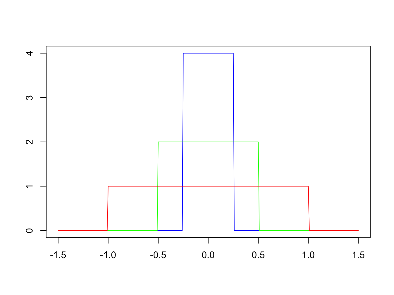
Figure 2.1: Graph of \(f_k(x)\) for \(k = 1\) (green), \(k = 2\) (red) and \(k =4\) (blue).
Sifting property of the delta function The delta function is most useful in how it interacts with other functions. Consider \[ \int_{-\infty}^{\infty} g(x) \delta(x) \, dx,\] where \(g(x)\) is a continuous function defined over \((-\infty, \infty)\). Using our definition of the delta-function we can rewrite this as
\[\begin{align*} \lim_{k \rightarrow \infty} \int^\infty_{-\infty} g(x) f_k(x) \, dx & = \lim_{k \rightarrow \infty} \int^{1/k}_{-1/k} \frac{k}{2} g(x) \, dx\\ & = \lim_{k \rightarrow \infty} \frac{k}{2} g(\bar{x}) \left(\frac{1}{k} - \left(-\frac{1}{k} \right) \right), \end{align*}\]
for some \(\bar{x}\) in \([-1/k, 1/k]\), using the mean-value theorem for integrals. Clearly, as \(k \rightarrow \infty\), we must have \(\bar{x} \rightarrow 0\). The expression above simplifies to
\[g(0) \frac{k}{2} \frac{2}{k} = g(0).\]
We have therefore established that for any continuous function \(g\):
\[\int_{-\infty}^{\infty} g(x)\delta(x) \, dx = g(0).\]
This result can easily be generalized to
\[\int_{-\infty}^{\infty} g(x)\delta(x -a) \, dx = g(a).\]
Using the definition of \(\cos \omega_0 x\) in terms of exponentials we have: \[\begin{align*} \mathcal{F}\{\cos \omega_0 x\} &= \int^\infty_{-\infty} \frac{1}{2} (e^{i\omega_0 x} + e^{-i\omega_0 x}) e^{-i\omega x} \,dx \\ & = \frac{1}{2} \int^\infty_{-\infty} e^{-i(\omega -\omega_0) x} \,dx+ \frac{1}{2} \int^\infty_{-\infty} e^{-i(\omega +\omega_0) x} \,dx \\ & = \pi \delta(\omega - \omega_0) + \pi \delta(\omega + \omega_0), \end{align*}\] which is a two-spiked ‘function’.
We finish by recommending this video on a very intuitive visual introduction to Fourier transform from the popular 3Blue1Brown YouTube channel in mathematics education. Do check it out and also the additional videos on related topics such as uncertainty principle.