Chapter 6 Introduction to Systems of ODEs
So far we have discussed ordinary differential equations where the function we have been looking for was a scaler function (\(y(x): \mathbb{R} \rightarrow \mathbb{R}\)). Where the unknown function is a vector (\(\vec{y}(x): \mathbb{R} \rightarrow \mathbb{R}^n\)), we are dealing with systems of ODEs.
Definition Systems of Ordinary Differential Equations have the following general form:
\[G_1(x, y_1, y_2, \cdots, y_n, \frac{dy_1}{dx}, \cdots, \frac{dy_n}{dx}, \cdots, \frac{d^{k_1}y_1}{dx^{k_1}}, \cdots, \ \frac{d^{k_n} y_n}{dx^{k_n}}) = 0,\]
\[\vdots\]
\[G_n(x, y_1, y_2, \cdots, y_n, \frac{dy_1}{dx}, \cdots, \frac{dy_n}{dx}, \cdots, \frac{d^{k_1}y_1}{dx^{k_1}}, \cdots, \ \frac{d^{k_n} y_n}{dx^{k_n}}) = 0.\]
The system is ordinary as we still have one independent variable \(x\), but now in contrast to single ODEs, we have \(n\) functions of independent variables \(y_1(x), y_2(x), \cdots, y_n(x)\) to solve for. This is the implicit form but the systems of ODEs can be written in explicit from as well. Many problems in physics and biology give rise to systems of ODEs. Here are few examples:
These models can be used to predict the dynamics of predator and prey systems such as rabbits (\(x(t)\)) and foxes (\(y(t)\)). A classic model is Lotka-Volterra model (1925/26) that can exhibit a periodic solution of the population of predator and preys as one goes up and the other goes down.
\[\begin{align*} \frac{dx}{dt} &= ax - bxy,\\ \frac{dy}{dt} &= dxy - cy. \end{align*}\]
The chemical rate equations for a set of chemical reactions. For example, consider the reversible binary reaction \(A + B \rightleftharpoons C\) with forward rate of \(k_1\) and backward rate of \(k_2\). We have the following rate equations for the concentrations \([A]\), \([B]\) and \([C]\).
\[\begin{align*} \frac{d[A]}{dt} = \frac{d[B]}{dt} &= k_2 [C] - k_1[A][B],\\ \frac{d[C]}{dt} = - \frac{d[A]}{dt}&= -k_2 [C] + k_1[A][B]. \end{align*}\] These kind of equations are used in mathematical modelling of biochemical reaction networks in systems and synthetic biology.
This is an example from mechanics. Consider the system of 3 masses and 4 springs that are fixed between two walls. We can write equations of motions that describe the position of the 3 masses as a function of time (\(x_1(t)\), \(x_2(t)\) and \(x_3(t)\)) as seen in Figure 6.1.
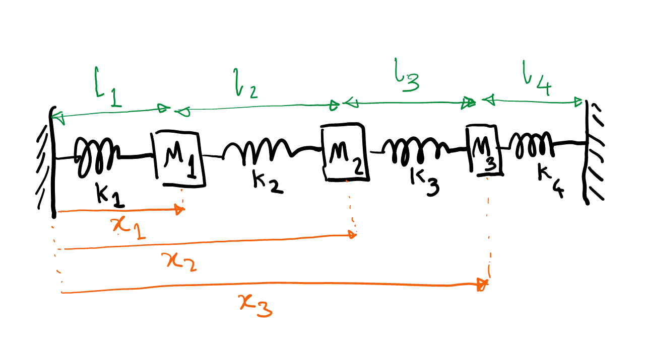
Figure 6.1: Diagram of the mass and spring system
Using the second Newton law for each mass (\(F = ma\)) and the Hook’s law (\(F = -k \Delta x\)) for the springs and given the relaxed lengths of each spring (\(l_1\) to \(l_4\)), and assuming the distance between the walls is the sum of the the relaxed lengths of the springs, we have the following system of ODEs:
\[\begin{align*} \frac{d^2x_1}{dt^2} &= - k_1 (x_1 - l_1) + k_2(x_2 - x_1 - l_2),\\ \frac{d^2x_2}{dt^2} &= - k_2 (x_2 - x_1 - l_2) + k_3(x_2 - x_2 - l_3),\\ \frac{d^2x_3}{dt^2} &= - k_3 (x_3 - x_2 - l_3) + k_4(l_1 + l_2 + l_3 - x_3). \end{align*}\]
One of the simplest but influential models of an epidemic is the compartmental SIR model. In this model, disease propagates between the population compartments through susceptible individuals (\(S\)) becoming infected (\(I\)) after encountering other infected individuals with rate \(\beta\) and finally moving to a recovered population (\(R\)) with rate \(\gamma\). The following simple system of ODEs describes the dynamics of this compartmental model.
\[\begin{align*} \frac{dS}{dt} &= - \beta SI,\\ \frac{dI}{dt} &= \beta SI - \gamma I,\\ \frac{dR}{dt} &= \gamma I. \end{align*}\]
This model and its variations are the basis of a lot of mathematical modelling that has been performed for predicting the effect of different interventions in the Covid-19 world-wide pandemic. If you like to learn a bit more about the SIR ODE system above check out this video. Also, the SIR model can be modeled using a so-called agent-based stochastic approach, where the individuals and their random interactions are specifically followed. You can check out this interesting video from the 3blue1brown series to see some cool exploration of this approach to SIR models.
6.1 Systems of first order ODEs
Systems of ODEs of general order can be rewritten in terms of systems of first order ODEs, so the following system written in explicit form is more general than it seems.
\[\frac{dy_1}{dx} = F_1(x, y_1, y_2, \cdots, y_n),\] \[\vdots\] \[\frac{dy_n}{dx} = F_n(x, y_1, y_2, \cdots, y_n).\]
The following second order ODE is the equation of motion for damped harmonic oscillator for a mass \(m\) that is attached to an ideal spring which follows the Hook’s law (\(F_S = - kx\), where \(x\) is position of the mass measured from the spring relaxed position) and has a damping friction force that is propotional and opposite in direction to its velocity \(F_D = - \eta \frac{dx}{dt}\) and is acted on by a deriving force \(F(t)\).
\[ m\frac{d^2x}{dt^2} + \eta \frac{dx}{dt} + kx = F(t).\]
By defining new variable \(u = dx/dt\) as the velocity of the mass \(m\), we can turn this second order ODE to a system of two first order ODEs:
\[\begin{align*}
\frac{dx}{dt} &= u,\\
\frac{du}{dt} &= \frac{1}{m}[F(t)- \eta u - kx].
\end{align*}\]
We can use a general vector notation to write systems of 1st order ODEs as \[\frac{d\vec{y}_{n \times 1}}{dt} = \vec{F}_{n \times 1}(t, \vec{y}_{n \times 1} ).\]
Here \(n\) is the number of equations, \(t\) is the independent variable and \(\vec{y}\) is the function we are looking for. In the next section, we discuss an important subclass of these systems.
6.2 Systems of linear 1st order ODEs with constant coefficients
Systems of linear 1st order ODEs with constant coefficients is an important class that we will discuss their solutions in detail. They have the following general form. \[\begin{align*} \frac{dy_1}{dt} &= \sum_{i=1}^n \alpha_{1i}y_i + g_1(t),\\ & \vdots\\ \frac{dy_n}{dt} &= \sum_{i=1}^n \alpha_{ni}y_i + g_n(t), \end{align*}\] where \(\alpha_{ij} \in \mathbb{R}\) are the constant coefficients forming the matrix \(A_{n \times n}\). We can write the system of linear ODEs in matrix form: \[\begin{bmatrix} \frac{dy_1}{dt} \\ \frac{dy_2}{dt} \\ \vdots \\ \frac{dy_n}{dt} \end{bmatrix} = \begin{bmatrix} \alpha_{11} & \alpha_{12} & \dots & \alpha_{1n} \\ \alpha_{21} & \alpha_{22} & \dots &\alpha_{2n} \\ \vdots & \vdots & \ddots & \vdots \\ \alpha_{n1} & \alpha_{n2} & \dots & \alpha_{nn} \end{bmatrix} \begin{bmatrix} y_1 \\ y_2 \\ \vdots \\ y_n \end{bmatrix} + \begin{bmatrix} g_1(t) \\ g_2(t) \\ \vdots \\ g_n(t) \end{bmatrix}. \] We can write this briefly as \[\frac{d\vec{y}}{dt} = A \vec{y} + \vec{g}(t).\]
Now if we define the linear operator \(\mathcal{L}[\vec{y}] = [\frac{d}{dt} - A]\vec{y}\) then we can write the system of linear first order ODEs as \[\mathcal{L}[\vec{y}] = \vec{g}(t).\]
Since both matrix \(A\) and derivative \(\frac{d}{dt}\) are linear operators, the operator associated to systems of linear ODEs \(\mathcal{L}\) is also a linear operator. By linearity we have: \[\mathcal{L}[\lambda_1\vec{y_1} + \lambda_2\vec{y_2}] = \lambda_1 \mathcal{L}[\vec{y_1}] + \lambda_2 \mathcal{L}[\vec{y_2}].\] Therefore, the solutions of the homogenous systems of \(n\) linear ODEs \(\mathcal{L}[\vec{y}_H] = 0\) forms a vector space of dimension \(n\). So a set of linearly independent solutions \(B = \{\vec{y}_i\}_{i=1}^n\) form a basis for this space. Therefore, similar to linear ODEs, the general solution can be written as \[\vec{y}^H_{GS} = \sum_{i=1}^n c_i \vec{y}_i,\] where \(c_i\)s are \(n\) arbitrary constants of integration.
The general solution of non-homogenous systems of 1st order linear ODEs
Similar to the case of linear ODEs, here also we find the general solution in two steps
Obtain complimentary function \(\vec{y}_{CF}\) by solving the corresponding homogenous systems of ODEs (\(\mathcal{L}[\vec{y}_{CF}] = 0\))
Find a particular integral \(\vec{y}_{PI}\) that satisfies the full non-homogenous systems of ODEs (\(\mathcal{L}[\vec{y}_{PI}] = \vec{g}(t)\)).
Then, for the general solution \(\vec{y}_{GS}\) we have: \[\vec{y}_{GS}(t; c_1, c_2, \cdots, c_n) = \vec{y}_{CF} + \vec{y}_{PI}.\]
Solving the homogenous problem
\[\mathcal{L}[\vec{y}_H] = 0 \quad \Longrightarrow \quad \frac{d\vec{y}_H}{dt} = A \vec{y}_H\] First, we consider the case where matrix \(A\) has \(n\) distinct roots and therefore is diagonalizable.
That means that there exists a matrix \(V\) where, we have: \[V^{-1}AV = \Lambda = \begin{bmatrix} \lambda_1 & 0 & 0\\ 0 & \ddots & 0 \\ 0 & 0 & \lambda_n \end{bmatrix}.\]
where, \(i\)th column of the matrix \(V\) is the eigenvector of matrix \(A\) corresponding to the eigenvalue \(\lambda_i\): \[A \vec{v}_i = \lambda_i \vec{v}_i.\]
We use the eigenvectors matrix \(V\) to obtain the solution of the homogenous system. \[ \frac{d\vec{y}}{dt} = A \vec{y} \quad \Longrightarrow \quad V^{-1}\frac{d\vec{y}}{dt} = V^{-1}A VV^{-1} \vec{y}.\] Letting \(\vec{z} = V^{-1}\vec{y}\), we can write the system of ODEs as \[\frac{d\vec{z}}{dt} = \Lambda \vec{z}.\] The \(i\)th row of this equation gives us \(\frac{dz_i}{dt} = \lambda_i z_i\), which can be solved, so we obtain: \[\vec{Z} = \begin{bmatrix} c_1 e^{\lambda_1 t} \\ c_2 e^{\lambda_2 t} \\ \vdots \\ c_n e^{\lambda_n t} \end{bmatrix} \quad \Longrightarrow \quad \vec{y}_H = V \vec{Z} = \begin{bmatrix} \vdots & \vdots & & \vdots \\ \vec{v}_1 & \vec{v}_2 & \cdots & \vec{v}_n \\ \vdots & \vdots & & \vdots \end{bmatrix} \begin{bmatrix} c_1 e^{\lambda_1 t} \\ c_2 e^{\lambda_2 t} \\ \vdots \\ c_n e^{\lambda_n t} \end{bmatrix}.\] Therefore, we obtain the general solution of the homogenous system of first order linear ODEs to be: \[\vec{y}_{CF} = \vec{y}^H_{GS} = c_1 e^{\lambda_1 t}\vec{v}_1 + c_2 e^{\lambda_2 t}\vec{v}_2 + \cdots + c_n e^{\lambda_n t}\vec{v}_n. \] Finding particular integrals
\[\mathcal{L}[\vec{y}_{PI}] = \vec{g}(t).\] We will use Ansatz and use the methods of undetermined coefficients and variation of parameters as done for the linear ODEs.
\[\begin{align*} \dfrac{dx}{dt} &= -4x -3y -5, \\ \dfrac{dy}{dt} &= 2x + 3y - 2. \end{align*}\]
We can write this ODE in vector form as: \[\frac{d\vec{y}}{dt} = A\vec{y} + \vec{g}(t) = \begin{bmatrix} -4 & -3 \\ 2 & 3 \end{bmatrix} \begin{bmatrix} x \\ y \end{bmatrix} + \begin{bmatrix} -5 \\ -2 \end{bmatrix}.\]
First step is to obtain \(\vec{y}_{CF}\). We obtain the eigenvalues \(\lambda_1\) and \(\lambda_2\) and eigenvectors \(\vec{v}_1\) and \(\vec{v}_2\).
\[ \lambda^2 + \lambda - 6 = 0 \quad \Longrightarrow \quad \lambda_1 = 2, \, \lambda_2 = -3.\] We have the corresponding eigenvectors: \[\vec{v_1} = \begin{bmatrix} 1\\ -2 \end{bmatrix}, \quad \vec{v_2} = \begin{bmatrix} 3\\ -1 \end{bmatrix}.\]
\[ \vec{y}_{CF} = \vec{y}^H_{GS}(t; c_1, c_2) = c_1 e^{2t}\begin{bmatrix} 1 \\ -2 \end{bmatrix} + c_2 e^{-3t}\begin{bmatrix} 3 \\ -1 \end{bmatrix}.\]
2nd step is to find any particular integral \(\vec{y}_{PI}(t)\)} that satisfies:
\[\mathcal{L}[\vec{y}_{PI}] = \vec{g}(t) = \begin{bmatrix} -5 \\ -2 \end{bmatrix}.\] We use the ansatz: \[\vec{y}_{PI} = \begin{bmatrix} a \\ b \end{bmatrix}.\] By plugging the ansatz into the ODE we obtain the undetermined coefficients \(a\) and \(b\): \[ \vec{y}_{PI} = \begin{bmatrix} a \\ b \end{bmatrix} = A^{-1} \begin{bmatrix} 5 \\ 2 \end{bmatrix} = -\frac{1}{6} \begin{bmatrix} 3 & 3 \\ -2 & -4 \end{bmatrix}\begin{bmatrix} 5 \\ 2 \end{bmatrix} = \begin{bmatrix} -7/2 \\ 3 \end{bmatrix}.\] So we have: \[\vec{y}_{GS}(t; c_1, c_2) = \vec{y}_{CF} + \vec{y}_{PI} = c_1 e^{2t}\begin{bmatrix} 1 \\ -2 \end{bmatrix} + c_2 e^{-3t}\begin{bmatrix} 3 \\ -1 \end{bmatrix} + \begin{bmatrix} -7/2 \\ 3 \end{bmatrix}.\]
This is a second order linear ODE and we can solve it using the methods discussed in the last chapter. Using the ansatz \(e^{\lambda t}\), we obtain the following characteristic equation: \[m \lambda^2 + \eta \lambda + k = 0 \quad \Rightarrow \quad \lambda_{1,2} = \frac{-\eta \pm \sqrt{\eta^2 - 4km}}{2m}.\] If the roots are distinct we obtain: \[x_{GS} = c_1 e^{\lambda_1 t} + c_2 e^{\lambda_2 t}.\]
Alternatively, we can transform the second order ODE to systems of first order ODEs as seen before: \[\begin{align*} \dfrac{dx}{dt} &= u, \\ \dfrac{du}{dt} &= -\dfrac{\eta}{m} u - \dfrac{k}{m} x. \end{align*}\] We obtain the same \(\lambda_{1,2}\) as above for the eigenvalues of corresponding matrix \(A\) for this system of ODEs.
For the eigenvectors (\(\vec{v}_1\) and \(\vec{v}_2\)) of \(A\), we have:
\[\vec{v}_1: \quad A \vec{v}_1 = \lambda_1 \vec{v}_1 \quad \Longrightarrow \quad \begin{bmatrix} 0 & 1\\ -\frac{k}{m} & -\frac{\eta}{m} \end{bmatrix}\begin{bmatrix} v_{1x} \\ v_{1u} \end{bmatrix} = \lambda_1 \begin{bmatrix} v_{1x} \\ v_{1u} \end{bmatrix},\]
\[ v_{1u} = \lambda_1 v_{1x} \quad \Longrightarrow \quad \vec{v}_1 = \begin{bmatrix} 1 \\ \lambda_1 \end{bmatrix}.\] Similarly, we obtain for the second eigenvector: \[\vec{v}_2: \quad A \vec{v}_2 = \lambda_2 \vec{v}_2 \quad \Longrightarrow \quad \vec{v}_2 = \begin{bmatrix} 1 \\ \lambda_2 \end{bmatrix}.\]
This gives us the following general solution: \[\vec{y}_{GS} = \begin{bmatrix} x_{GS} \\ u_{GS} \end{bmatrix} = c_1 e^{\lambda_1 t} \begin{bmatrix} 1 \\ \lambda_1 \end{bmatrix} + c_2 e^{\lambda_2 t} \begin{bmatrix} 1 \\ \lambda_2 \end{bmatrix},\] which gives us the same general solution for \(x_{GS}\) as obtained using the previous method.
When \(A\) has repeated eigenvalues
Case 1: \(A\) is still diagonalizable (it has \(n\) linearly independent eigenvectors). Then we can still use the method described. For example for \(n = 2\) we have: \[A = \begin{bmatrix} \lambda & 0\\ 0 & \lambda \end{bmatrix} \quad \Rightarrow \quad \vec{v}_1 = \begin{bmatrix} 1\\ 0 \end{bmatrix}, \quad \vec{v}_2 = \begin{bmatrix} 0\\ 1 \end{bmatrix}.\] So, we have \[\vec{y}_{CF} = c_1 e^{\lambda t} \begin{bmatrix} 1\\ 0 \end{bmatrix} + c_2 e^{\lambda t} \begin{bmatrix} 0\\ 1 \end{bmatrix}.\]
Case 2: \(A\) is not diagonalizable (it has less than \(n\) linearly independent eigenvectors). Then we will use the Jordan normal form. We first discuss an example and then see the general case.Matrix \(A\) in this case has repeated roots: \[(1-\lambda)(3 - \lambda) + 1 = 0 \quad \Rightarrow \quad \lambda_1 = \lambda_2 = 2.\]
We next find the Eigenvector(s):
\[A \vec{v}_1 = \lambda_1 \vec{v}_1 \quad \Longrightarrow \quad \begin{bmatrix} 1 & -1 \\ 1 & 3 \end{bmatrix} \begin{bmatrix} v_{1x} \\ v_{1y} \end{bmatrix} = 2 \begin{bmatrix} v_{1x} \\ v_{1y} \end{bmatrix}.\]
Which gives us:
\[v_{1x} = - v_{1y} \quad \Rightarrow \quad \vec{v}_1 = \begin{bmatrix} 1 \\ -1 \end{bmatrix}.\]
So, this matrix only has one eigenvector and the matrix is not diagonalizable.
We look for similarity transformation to a Jordan normal form (\(J\); an almost diagonal form as defined below). We look for a matrix of the form: \[\quad \quad \quad \quad \quad W = \begin{bmatrix} 1 & \alpha \\ -1 & \beta \end{bmatrix}.\] So that: \[W^{-1}AW = \begin{bmatrix} 2 & 1 \\0 & 2 \end{bmatrix} = J,\] where, \(J\) is the Jordan normal form for a 2 by 2 matrix. We have: \[Aw = w\begin{bmatrix} 2 & 1 \\0 & 2 \end{bmatrix} \quad \Rightarrow \quad \begin{bmatrix} 1 & -1 \\1 & 3 \end{bmatrix} \begin{bmatrix} 1 & \alpha \\-1 & \beta \end{bmatrix} = \begin{bmatrix} 1 & \alpha \\-1 & \beta \end{bmatrix} \begin{bmatrix} 2 & 1 \\0 & 2 \end{bmatrix}.\] So, we obtain the following equations for \(\alpha\) and \(\beta\). \[\begin{array}{rl} \alpha - \beta \,\,\, = & 1 + 2\alpha \\ \alpha + 3 \beta \,\,\, = & - 1 + 2\beta \end{array} \quad \Longrightarrow \quad \alpha + \beta = -1 \quad \Longrightarrow \quad \vec{w}_2 = \begin{bmatrix} 1 \\ -2 \end{bmatrix},\] giving us \[W = \begin{bmatrix} 1 & 1 \\-1 & -2 \end{bmatrix},\] and we can check that \(W^{-1}AW = J\). The Jordan normal form allows us to solve the non-diagonalizable systems of ODEs: \[\dfrac{d\vec{y}}{dt} = A \vec{y} \quad \Longrightarrow \quad W^{-1}\dfrac{d\vec{y}}{dt} = \left[W^{-1} A W\right] W^{-1}\vec{y}. \] Letting \(\vec{z} = W^{-1}\vec{y}\), we obtain \(\frac{d\vec{z}}{dt} = J \vec{z}\), so we have: \[\begin{array}{rl} \dfrac{dz_1}{dt} \,\,\, = & 2z_1 + z_2,\\ \dfrac{dz_2}{dt} \,\,\, = & 2z_2. \end{array} \] We can solve the second ODE to obtain \(z_2 = c_2 e^{2t}\) and we can then use this solution to solve for \(z_1\) from the first equation above: \[z_1 = c_1 e^{2t} + c_2 t e^{2t}.\] So in vector form: \[\vec{z}_{GS} = \begin{bmatrix} z_1 \\ z_2 \end{bmatrix} = \begin{bmatrix} c_1e^{2t} + c_2 t e^{2t} \\ c_2 e^{2t} \end{bmatrix}.\] Now we can obtain the general solution for \(\vec{y}_{GS}\). \[\vec{y}_{GS} = W \vec{z}_{GS} = \begin{bmatrix} \vec{v}_1 & \vec{w}_2 \end{bmatrix} \begin{bmatrix} c_1e^{2t} + c_2 t e^{2t} \\ c_2 e^{2t} \end{bmatrix} = (c_1e^{2t} + c_2 t e^{2t})\vec{v}_1 + c_2 e^{2t}\vec{w}_2.\]
The case of non-diagonalizable \(A_{n\times n}\) with one repeated eigenvalue \(\lambda\)
Assume \(\lambda\) is associated with only a single eigenvector. We can use the Jordan normal form (\(J\)) to obtain a solution to the associated systems of linear ODEs. We look for a similarity transformation \(W\) to transform \(A\) to \(J\): \[W^{-1}AW = J = \begin{bmatrix} \lambda & 1 & 0 & 0 & 0 \\ 0 & \lambda & 1 & 0 & 0 \\ 0 & 0 & \ddots & 1 & 0 \\ 0 & 0 & 0 & \lambda & 1 \\ 0 & 0 & 0& 0& \lambda \end{bmatrix}. \] Letting \(\vec{z} = W^{-1}\vec{y}\), we obtain \(\frac{d\vec{z}}{dt} = J \vec{z}\), so we have: \[\begin{array}{rl} \dfrac{dz_n}{dt} \,\,\, = \lambda z_n \quad & \Rightarrow \quad z_n = c_ne^{\lambda t}\\ \dfrac{dz_{n-1}}{dt} \,\,\, = \lambda z_{n-1} + z_n \quad & \Rightarrow \quad z_{n-1} = c_{n-1}e^{\lambda t} + c_n t e^{\lambda t}\\ \dfrac{dz_{n-2}}{dt} \,\,\, = \lambda z_{n-2} + z_{n-1} \quad & \Rightarrow \quad z_{n-2} = c_{n-2}e^{\lambda t} + c_{n-1}t e^{\lambda t} + c_n \frac{t^2}{2} e^{\lambda t}\\ \vdots & \\ \dfrac{dz_{1}}{dt} \,\,\, = \lambda z_{1} + z_2 \quad & \Rightarrow \quad z_1 = c_1e^{\lambda t} + c_2 t e^{\lambda t} + \cdots + c_n \frac{t^{n-1}}{(n-1)!} e^{\lambda t}\\ \end{array} \] So, we can obtain \(\vec{y}_{GS} = W \vec{z}_{GS}\).
There could be situations where the matrix has some distinct eigenvalues and some repeated eigenvalues, which will result in different Jordan normal forms. For example, consider a matrix \(A_{3 \times 3}\) with two distinct eigenvalues one repeated. The suitable Jordan normal form would have the following form: \[J = \begin{bmatrix} \lambda_1 &1 & 0 \\ 0 & \lambda_1 & 0 \\ 0 & 0& \lambda_2 \end{bmatrix}.\]