Chapter 1 Fourier Transforms
Last term, we saw that Fourier series allows us to represent a given function, defined over a finite range of the independent variable, in terms of sine and cosine waves of different amplitudes and frequencies. Fourier Transforms are the natural extension of Fourier series for functions defined over \(\mathbb{R}\). A key reason for studying Fourier transforms (and series) is that we can use these ideas to help us solve differential equations as seen in this course regarding ordinary differential equations and more extensively next year in relation to partial differential equations. There are also many other applications for Fourier transforms in science and engineering, particularly in the context of signal processing.
1.1 Fourier’s integral formula
We can represent a function \(f(x)\) defined over the interval \([-L, L]\) using the Fourier series
\[f(x) = \frac{1}{2} a_0 + \sum_{n=1}^{\infty} \{ a_n \cos\left( {\frac{n\pi x}{L}}\right) + b_n \sin\left( {\frac{n\pi x}{L}}\right) \}.\] where the corresponding Fourier coefficients are given by \[ a_n = \frac{1}{L} \int_{-L}^{L} f(x) \cos\left( {\frac{n\pi x}{L}}\right) dx, \quad n = 0, 1, 2, \cdots, \] \[ b_n = \frac{1}{L} \int_{-L}^{L} f(x) \sin\left( {\frac{n\pi x}{L}}\right) dx, \quad n = 1, 2, \cdots. \] Expressed in the exponential form the Fourier series can be represented as \[f(x) = \sum_{n=-\infty}^{\infty} c_n e^{i n\pi x/L}, \quad |x| < L, \] \[ c_n = \frac{1}{2L} \int_{-L}^{L} f(x) e^{- i n\pi x/L} \, dx, \quad n = 0, \pm 1, \pm2, \cdots.\]
By defining angular frequency as \(\omega_n = n\pi/L\) and frequency difference as \[\delta \omega = \omega_{n+1} - \omega_{n},\] we can rewrite the Fourier series in the new notation as \[f(x) = \frac{1}{2\pi} \sum^\infty_{n = -\infty} \left[ \int_{-L}^L f(s) e^{-i\omega_n s} ds \right] e^{-i\omega_n x} \delta \omega.\]
This result can be extended for a function \(f(x)\) defined on \(\mathbb{R}\) by taking the limit of \(L \rightarrow \infty\) from the Fourier series. Using the angular frequency notation from above and replacing sum with integral using the Riemann sum, noting that \(\delta \omega \rightarrow 0\) as \(L \rightarrow \infty\) , we obtain \[f(x) = \frac{1}{2\pi} \int_{-\infty}^{\infty} \left\lbrace \int_{-\infty}^{\infty} f(s) e^{-i \omega s} \, ds \right\rbrace e^{i \omega x} \, d\omega.\] We therefore have shown that for a function \(f(x)\) defined over \(-\infty < x < \infty\) we have the following \[f(x) = \frac{1}{2\pi} \int_{-\infty}^{\infty} \hat{f}(\omega) e^{i \omega x} \, d\omega,\] where \[\hat{f}(\omega) = \int_{-\infty}^{\infty} f(x) e^{-i \omega x} \, dx.\] The function \(\hat{f}(\omega)\) (also denoted as \(\mathcal{F}\{f(x)\}\)) is known as Fourier transform of \(f(x)\), which is analogous to the Fourier coefficients in a Fourier series. The relation above between \(f(x)\) and \(\hat{f}(\omega)\) is also known as inverse Fourier transform. Note that some books use slightly different definitions of Fourier transform with different normalisation. In order to evaluate the integrals above, a necessary condition is that \(f(x)\) and its transform decay at \(\pm \infty\). Using the Dirac delta function this restriction can be overcome as seen later.
Proof of Fourier’s integral formula
In the previous section in a non-rigorous way we arrived at the result
\[f(x) = \frac{1}{2\pi} \int_{-\infty}^{\infty} \left\lbrace \int_{-\infty}^{\infty} f(s) e^{-i \omega s} \, ds \right\rbrace e^{i \omega x} \, d\omega.\]
To prove this more formally, we need to assume that \(f(x)\) is such that
\[\int_{-\infty}^{\infty} | f(x)| \, dx\]
converges. We will also assume that \(f(x)\) and \(f'(x)\) are continuous for all \(x\) (this can be relaxed as discussed at the end). We start by writing the RHS above in the form \[\begin{align*} & \lim_{L \rightarrow \infty} \frac{1}{2\pi} \int_{-L}^{L} \left\lbrace \int_{-\infty}^{\infty} f(s) e^{-i\omega (s -x)} \, ds \right\rbrace \, d\omega = \\ & \lim_{L \rightarrow \infty} \frac{1}{2\pi} \int_{-L}^{L} \left\lbrace \int_{-\infty}^{\infty} f(s) \cos{[\omega (s -x)]} \, ds - i \int_{-\infty}^{\infty} f(s) \sin{[\omega (s -x)]} \, ds \right\rbrace \, d\omega. \end{align*}\]
The first integral in curly brackets is even about \(\omega = 0\), while the second is odd. Also, because of the absolute convergence of the inner integral, we can interchange the order of integration. Therefore, the expression simplifies to
\[\begin{align*} & \lim_{L \rightarrow \infty} \frac{1}{\pi} \int_{0}^{L} \left\lbrace \int_{-\infty}^{\infty} f(s) \cos{[\omega (s -x)]} \, ds \right\rbrace \, d\omega \\ = & \lim_{L \rightarrow \infty} \frac{1}{\pi} \int_{-\infty}^{\infty} f(s) \left\lbrace \int_{0}^{L} \cos{[\omega (s -x)]} \, d\omega \right\rbrace \, ds \\ = & \lim_{L \rightarrow \infty} \frac{1}{\pi} \int_{-\infty}^{\infty} f(s) \frac{\sin{[L(s -x)]}}{s-x} \, ds \\ = & \lim_{L \rightarrow \infty} \frac{1}{\pi} \int_{-\infty}^{\infty} f(x+u) \frac{\sin{(Lu)}}{u} \, du, \end{align*}\]
using the substitution \(u = s-x\). We now split the integral into two parts in the following form
\[\lim_{L \rightarrow \infty} \frac{1}{\pi} \left\lbrace \int_{-\infty}^{\infty} \frac{f(x+u) - f(x)}{u} \sin{(Lu)}\,du + f(x) \int_{-\infty}^{\infty} \frac{\sin{(Lu)}}{u} \, du \right\rbrace .\]
The first integral tends to zero as \(L \rightarrow 0\) using Riemann-Lebesgue Lemma (seen last term in this course). We then use the substitution \(p = Lu\) in the second integral to leave \[\lim_{L \rightarrow \infty} \frac{f(x)}{\pi} \int_{-\infty}^{\infty} \frac{\sin{(p)}}{p} \, dp = f(x),\] using the fact that \(\int_{-\infty}^{\infty} (\sin{p})/p \, dp = \pi\) (seen last term and also in the problem sheet 1 this term).
We have therefore proved Fourier’s integral formula. As remarked earlier, we have assumed here that \(f(x)\) is continuous at all \(x\). If there is a discontinuity at \(x_0\) (with finite left and right hand derivatives there), the LHS of the formula is replaced by \([f(x_0+) + f(x_0−)]/2\) (analogous to the Fourier series convergence we investigated earlier).
Example 1.1 Find the Fourier transform of the rectangular wave
\[ f(x) = \left\{ \begin{array}{rl} 1, & \text{if } |x| < d,\\ 0, & \text{if } |x| > d. \end{array} \right. \]Using the Fourier transform formula we have \[\hat{f}(\omega) = \int^d_{-d} 1.e^{-iwx} \, dx = \left[ \frac{e^{-i\omega x}}{-i\omega} \right]^d_{-d} = -\frac{1}{i\omega}(e^{-i\omega d} - e^{i \omega d}) = \frac{2}{\omega} \sin \omega d.\] See Figure 1.1 for a graph of \(\hat{f}(\omega)\) for different values of \(d\). Note that as \(d\) gets larger, \(\hat{f}\) becomes more concentrated in the vicinity of \(\omega = 0\). This is a general property of Fourier transforms and its inverse and relates to uncertainty principle. A function which is more localised around zero has a wider inverse Fourier transform. See unseen question 1 for the derivation and further discussion of the uncertainty principle.
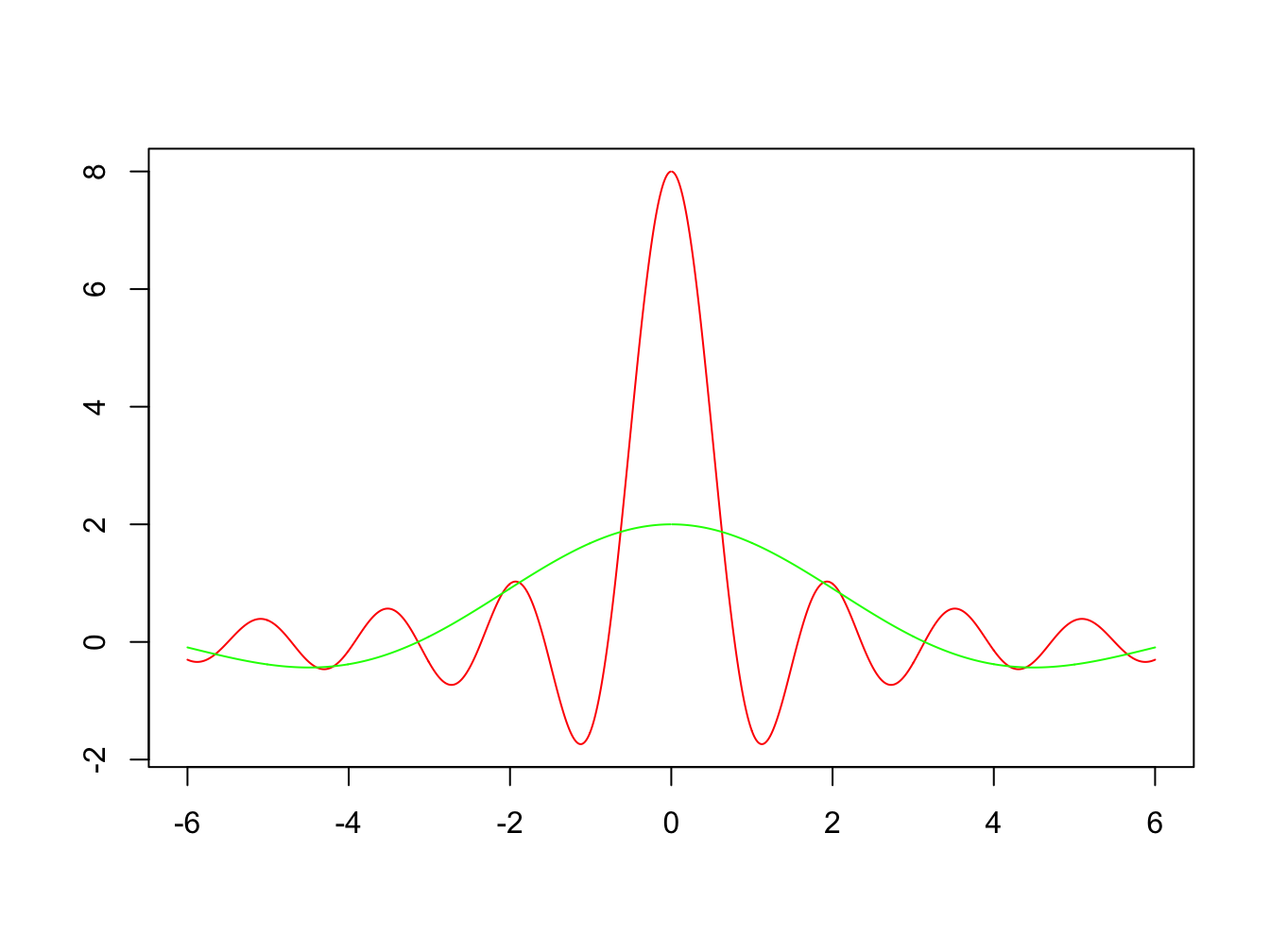
Figure 1.1: Graph of the Fourier transform for \(d = 1\) (green) and \(d = 4\) (red)
1.2 Fourier cosine and sine transforms
We can exploit the symmetry to define transforms over the range \([0, \infty)\). First, if we suppose that \(f(x)\) is even about \(x =0\), we have \[\begin{align*} \hat{f}(\omega) & = \int_{-\infty}^{\infty} f(x)e^{-i\omega x} \,dx = \int_{-\infty}^{\infty} f(x)(\cos{\omega x} - i \sin{\omega x}) \, dx \\ & = 2 \int_{0}^{\infty} f(x) \cos{\omega x} \, dx. \end{align*}\] We define Fourier cosine transform of \(f(x)\) to be \[ \hat{f}_c(\omega) = \int_{0}^{\infty} f(x) \cos{\omega x} \, dx.\] Thus, for an even function \(f(x)\) we have \(\hat{f}(\omega) = 2 \hat{f}_c(\omega)\).
Using the inversion formula for the regular transform and exploiting the evenness of \(\hat{f}_c(\omega)\), we can obtain the inversion formula for the Fourier cosine transform: \[f(x) = \frac{1}{2\pi} \int_{-\infty}^{\infty} \hat{f}(\omega) e^{i\omega x} \ d\omega = \frac{2}{\pi} \int_{0}^{\infty} \hat{f}_c(\omega) \cos \omega x \, d\omega.\]
In a similar way, by considering \(f(x)\) to be odd about \(x = 0\), we can define a Fourier sine transform and derive the corresponding inversion formula. We obtain the pair of expressions: \[\begin{align*} \hat{f}_s(\omega) & = \int_{0}^{\infty} f(x) \sin{\omega x} \, dx \\ f(x) & = \frac{2}{\pi} \int_{0}^{\infty} \hat{f}_s(\omega) \sin{\omega x} \, dw. \end{align*}\]
For an odd function \(f(x)\), we have \(\hat{f}(\omega) = -2i \hat{f}_s(\omega)\).
\[ f(x) = \left\{ \begin{array}{rl} 1, & \text{if } |x| < d,\\ 0, & \text{if } |x| > d. \end{array} \right. \]
We can use the definition of Fourier cosine transform directly noting that the function is even. But also, as we have already obtained the Fourier transform of this function in the last example, we simply have: \[\hat{f}_c(\omega) = \frac{1}{2}\hat{f}(\omega) = \frac{1}{\omega} \sin \omega d.\]