Chapter 5 Linear ODEs

The general form of linear ODEs of order $k$ is $$\alpha_k(x)\frac{d^ky}{dx^k} + \alpha_{k-1}(x)\frac{d^{k-1}y}{dx^{k-1}} + ... + \alpha_1(x)\frac{dy}{dx} + \alpha_0(x) y = f(x),$$ where $\alpha_k(x)$,.., $\alpha_0(x)$ and $f(x)$ are functions of only the independent variable $x$. The ODE is called homogeneous if $f(x) = 0$ and inhomogeneous otherwise.

Some examples of linear ODEs:

• First order ODE $$\frac{dy}{dx} + p(x)y = q(x).$$
• Bessel’s equation $$x^2 \frac{d^2y}{dx^2} + x \frac{dy}{dx} + (x^2 - n^2) y = 0.$$
• Legendre’s equation $$(1 -x^2) \frac{d^2y}{dx^2} - 2x \frac{dy}{dx} + n(n+1) y = 0.$$

Linear Operators

We define the differential operator as $\mathcal{D}[f] \equiv \frac{d}{dx}[f]$.

Differential operator is a linear operator since we have: $$\mathcal{D}[\lambda_1 f_1 + \lambda_2 f_2] = \lambda_1 \mathcal{D}[f_1] + \lambda_2 \mathcal{D}[f_2].$$ Defining differential operator of order $k$ as $\mathcal{D}^k[f] \equiv \frac{d^k}{dx^k}[f]$, which is also a linear operator as we have: $$\mathcal{D}^k[\lambda_1 f_1 + \lambda_2 f_2] = \lambda_1 \mathcal{D}^k[f_1] + \lambda_2 \mathcal{D}^k[f_2].$$ Linear ODEs are associated with a linear operator defined using the differential operators: $\mathcal{L}[y] \equiv \sum_{i=0}^{k} \alpha_i(x) \mathcal{D}^i[y]$ since: $$\mathcal{L}[\lambda_1 f_1 + \lambda_2 f_2] = \lambda_1 \mathcal{L}[f_1] + \lambda_2 \mathcal{L}[f_2].$$ A linear ODE can thus be simply written as $\mathcal{L}[y] = f(x)$ and a homogenous ODE as $\mathcal{L}[y] = 0$. Linearity of $\mathcal{L}$ has an important consequence. If we have two solutions $y_1$ and $y_2$ of a homogenous linear ODE $\mathcal{L}[y] = 0$, then any linear combinations of these solutions are also solutions for this ODE, since: $$\mathcal{L}[\lambda_1 f_1 + \lambda_2 f_2] = \lambda_1 \mathcal{L}[f_1] + \lambda_2 \mathcal{L}[f_2] = 0.$$

Linear independence

A set of functions $\{f_i(x)\}_{i=1}^k$ is said to be linearly independent if $f_i$’s satisfy the following condition: $$c_1 f_1(x) + c_2 f_2(x) + \cdots + c_k f_k(x) = 0,$$ if and only if $c_1 = c_2 = \cdots = c_k = 0$.

Linear ODEs are easier to solve because of the following important property of their solutions. This is a basic consequence of linearity of differential operators.

Proposition 5.1 The solutions of the homogeneous linear ODE $\mathcal{L}[y] = 0$ form a vector space (see MATH40003: Linear Algebra and Groups) of dimension $k$, where $k$ is the order of the ODE. Therefore, the general solution of a linear homogeneous ODE can be written as $$y_{GS}^H(x; c_1, ..., c_k) = c_1 y_1 + c_2 y_2 + ... + c_k y_k,$$ where $B = \{y_i(x)\}_{i = 1}^k$ is a set of linearly independent solutions forming a basis for the linear homogeneous ODE’s solution vector space.

Proposition 5.2 To test the linear independence of a set of functions $\{y_i(x)\}_{i = 1}^k$, we calculate the Wronskian, which is the determinant of the Wronskian matrix ($\mathbb{W}_{k\times k}$): $$W[\{y_i(x)\}_{i = 1}^k] = \text{det} \mathbb{W} = \text{det} \begin{bmatrix} y_1(x) & y_2(x) & \cdots & y_k(x) \\ \frac{dy_1}{dx}(x) & \frac{dy_2}{dx}(x) & \cdots & \frac{dy_k}{dx}(x) \\ \vdots & \vdots & & \vdots \\ & & & \\ \frac{d^{k-1}y_1}{dx^{k-1}}(x) & \frac{d^{k-1}y_2}{dx^{k-1}}(x) & \cdots & \frac{d^{k-1}y_k}{dx^{k-1}}(x) \end{bmatrix}$$ The set $\{y_i(x)\}_{i = 1}^k$ is linearly independent if $$W[\{y_i(x)\}_{i = 1}^k] \neq 0.$$

Proof We prove this by contradiction; If we assume $W(x) \neq 0$ but $\{y_i(x)\}_{i = 1}^k$ are linearly dependent:

$$\exists i \in \{1,\cdots, k\}, \quad c_i \neq 0, \quad \sum_{i=1}^k c_i y_i(x) = 0.$$

By taking derivatives repeatedly with respect to $x$ from the above equation we obtain:

$$\begin{align*} \sum_{i=1}^k c_i \frac{dy_i}{dx} & = 0\\ \vdots & \\ \sum_{i=1}^k c_i \frac{d^{k-1}y_i}{dx^{k-1}} & = 0, \end{align*}$$

which can be written as $\mathbb{W}.\vec{c} = 0$, with $\vec{c}$ defined as $$\vec{c} = \begin{bmatrix} c_1\\ \vdots \\ c_k \end{bmatrix},$$ since $\vec{c} \ne 0$ then $\mathbb{W}.\vec{c} = 0$ implies $W[\{y_i(x)\}_{i = 1}^k] = \text{det} \mathbb{W} = 0$, which is a contradiction. So, if $W(x) \ne 0$ then $\{y_i(x)\}_{i = 1}^k$ are linearly independent, as required.

Example 5.1 Show that $\sin(x)$ and $\cos(x)$ are linearly independent.

$$\mathbb{W}_{2 \times 2} = \begin{bmatrix} \sin(x) & \cos(x) \\ \cos(x) & \sin(x) \end{bmatrix},$$ then $$W(x) = \text{det} \mathbb{W} = - \sin^2(x) - \cos^2(x) = -1 \ne 0,$$ therefore $\sin(x)$ and $\cos(x)$ are linearly independent.

Note There exists examples in which the Wronskian vanishes without the functions being linearly dependent. An example is given in a quiz in the lectures.

5.1 General solution of the non-homogeneous linear ODE

To obtain the general solution of the non-homogeneous linear ODE $$\mathcal{L}[y] = f(x),$$ we split the problem into two simpler steps:

1. We consider the corresponding homogeneous linear ODE $\mathcal{L}[y] = 0$. We obtain the general solution, which is also known as complementary function ($y_{CF}$): $$y_{CF} = y_{GS}^H(x; c_1, \cdots, c_k) = \sum_{i=1}^{k} c_i y_i(x),$$ where, $\{y_i\}_{i=1}^k$ are the basis of the solution vector space (a set of linearly independent solutions of the homogeneous linear ODE).

2. We obtain any/one solution of the full non-homogeneous ODE, which is also known as particular integral ($y_{PI}$): $$\mathcal{L}[y_{PI}] = f(x).$$ Then for the solution to the full problem by combining the results above and due to linearity, we have:

$$\mathcal{L}[y_{GS}(x; c_1, \cdots, c_k)] = \mathcal{L}[y_{CF} + y_{PI}] = \mathcal{L}[y^H_{GS}] + \mathcal{L}[y_{PI}] = f(x).$$ So the general solution of the non-homogeneous linear ODE is the sum of the complementary function and a particular integral. As seen in a quiz in the lectures different choices of particular integrals results in the same family of general solutions.

One useful consequence of the linearity is that if the RHS of the ODE is sum of two functions: $$\mathcal{L}[y] = f_1(x) + f_2(x).$$ We can break the second step of finding particular integral into additional steps.

1. Find $y_{CF} = y^H_{GS}(x; c_1, \cdots, c_k)$ such that $\mathcal{L}[y_{CF}] = 0$.

2. Find any solution to $\mathcal{L^1_{PI}}[y] = f_1(x)$.

3. Find any solution to $\mathcal{L^2_{PI}}[y] = f_2(x)$.

Then, we have $y_{GS} = y_{CF} + y^1_{PI} + y^2_{PI}$.

Linear ODEs with constant coefficients

The general linear ODE is not always analytically solvable. Next year, you will see approximative and numerical methods to solve this kind of ODEs. In the rest of this course, we will focus on the case of linear ODEs with constant coefficients ($\alpha_i$s not depending on independent variable $x$): $$\mathcal{L}[y] = \sum_{i=0}^{k} \alpha_i \mathcal{D}^i[y] = f(x)$$

5.2 First order linear ODEs with constant coefficients

The general form of the first order linear ODEs with constant coefficients is: $$\mathcal{L}[y] = \alpha_1 \frac{dy}{dx} + \alpha_0 y = f(x).$$ As seen in chapter 4, rewriting this ODE as $$\frac{dy}{dx} + \frac{\alpha_0}{\alpha_1}y = \frac{f(x)}{\alpha_1},$$

we can obtain the general solution using the integrating factor $I(x) = e^{\frac{\alpha_0}{\alpha_1} x}$. We obtain

$$y_{GS} = c_1 e^{-\frac{\alpha_0}{\alpha_1}x} + e^{-\frac{\alpha_0}{\alpha_1}x} \int e^{\frac{\alpha_0}{\alpha_1}x}\frac{f(x)}{\alpha_1} \, dx.$$

Example 5.2 Solve $f(x) = x$.

Using the general solution above, and by integration by parts, we obtain: $$y_{GS} = c_1 e^{-\frac{\alpha_0}{\alpha_1}x} + \left[ \frac{x}{\alpha_0} - \frac{\alpha_1}{\alpha_0^2} \right].$$

Alternative method

1. Solve the corresponding homogeneous ODE: $$\mathcal{L}[y_{CF}] = \alpha_1 \frac{dy}{dx} + \alpha_0 y = 0.$$ This is a separable ODE and by integration we obtain: $$y_{CF} = y^H_{GS}(x; c_1) = c_1 e^{-\frac{\alpha_0}{\alpha_1}x}.$$
2. Find a particular integral for the full ODE: $\mathcal{L}[y_{PI}] = f(x) = x$.

This is done by using ansatz, which is an educated guess using the method of undetermined coefficients. In this case as $f(x)$ is polynomial, we could try a polynomial ansatz: $$y_{PI} = Ax^2 + Bx + C,$$ where, $A$, $B$ and $C$ are constants to be determined. By plugging this ansatz in to the ODE, we check if here are suitable values for these constants that makes our ansatz a particlular solution for the ODE: $$\mathcal{L}[y_{PI}] = \alpha_1(2Ax + B) + \alpha_0(Ax^2 + Bx + C) = x.$$ This equation should be satisfied for all $x \in \mathbb{R}$, so we equate the coefficients of the powers of $x$: $$\begin{align*} x^2: & \quad \alpha_0 A = 0 \quad \Rightarrow \quad A = 0;\\ x^1: & \quad 2\alpha_1 A + \alpha_0 B = 1 \quad \Rightarrow \quad B = \frac{1}{\alpha_0};\\ x^0: & \quad \alpha_1 B + \alpha_0 C = 0 \quad \Rightarrow \quad C = -\frac{\alpha_1}{\alpha_0^2}, \end{align*}$$ which gives us the same general solution obtained using the first method: $$y_{GS} = y_{CF} + y_{PI} = c_1 e^{-\frac{\alpha_0}{\alpha_1}x} + \left[ \frac{x}{\alpha_0} - \frac{\alpha_1}{\alpha_0^2} \right].$$

Example 5.3 Solve $f(x) = e^{bx}; b \neq -\frac{\alpha_0}{\alpha_1}$.

The ODE is the following:
$$\mathcal{L}[y] = \alpha_1 \frac{dy}{dx} + \alpha_0 y = e^{bx}.$$ Using the two step method, we have as before:

1. $y_{CF} = y^H_{GS}(x; c_1) = c_1 e^{-\frac{\alpha_0}{\alpha_1}x}.$

2. We try ansatz $y_{PI} = A e^{bx}$, plugging this into the ODE, we obtain: $$\alpha_1 Ab e^{bx} + \alpha_0 A e^{bx} = e^{bx}.$$ Solving this we obtain $A = \frac{1}{\alpha_1b + \alpha_0}$. So we obtain: $$y_{GS} = y_{CF} + y_{PI} = c_1 e^{-\frac{\alpha_0}{\alpha_1}x} + \frac{1}{\alpha_1 b + \alpha_0} e^{bx}.$$ What about the case $b = -\frac{\alpha_0}{\alpha_1}$? Naive ansatz $y_{PI} = A e^{bx}$ does not work, since $\mathcal{L}[y_{PI}] = 0$. A more general ansatz is: $$y_{PI} = A(x)e^{bx}.$$ Here we are looking for an unknown function $A(x)$, so we will obtain an ODE. This is called the method of variation of parameters, developed by Euler and Lagrange. Plugging this ansatz into the ODE we obtain the following simple ODE: $$\alpha_1 \frac{dA}{dx} = 1,$$ which has the following general solution: $$A(x) = \frac{x}{\alpha_1} + c_2.$$ So, we obtain for the general solution: $$y_{GS} = y_{CF} + y_{PI} = c_1 e^{-\frac{\alpha_0}{\alpha_1}x} + (\frac{x}{\alpha_1} + c_2) e^{bx} = c' e^{-\frac{\alpha_0}{\alpha_1}x} + \frac{x}{\alpha_1} e^{bx},$$ where in the last step we have renamed $c_1 + c_2$ as $c'$ a new constant of integration.

5.3 Second order linear ODEs with constant coefficients

$$\mathcal{L}[y] = \alpha_2 \frac{d^2y}{dx^2} + \alpha_1 \frac{dy}{dx} + \alpha_0 y = f(x),$$ $$y_{GS}(x; c_1, c_2) = y_{CF}(x; c_1, c_2) + y_{PI} = y^H_{GS}(x; c_1, c_2) + y_{PI}.$$ If $B = \{y_1(x), y_2(x)\}$ is a basis for the solution vector space of the homogeneous ODE: $\mathcal{L}[y^H] = 0$. Then, we have: $$y^H_{GS}(x; c_1, c_2) = c_1 y_1(x) + c_2 y_2(x).$$

Solving the homogeneous second order linear ODE

We need to obtain two linearly independent solutions to the following ODE:

$$\mathcal{L}[y] = \alpha_2 \frac{d^2y}{dx^2} + \alpha_1 \frac{dy}{dx} + \alpha_0 y = 0.$$

We can try the ansatz: $y^H = e^{\lambda x}$,

$$\mathcal{L}[y^H] = \alpha_2 \lambda^2 e^{\lambda x} + \alpha_1 \lambda e^{\lambda x} + \alpha_0 e^{\lambda x} = 0 \quad \Rightarrow \quad \alpha_2 \lambda^2 + \alpha_1 \lambda + \alpha_0 = 0.$$ This quadratic equation is called the characteristic equation of the linear ODE, which has the following solutions: $$\lambda_1, \lambda_2 = \frac{-\alpha_1 \pm \sqrt{\alpha_1^2 - 4 \alpha_0 \alpha_2}}{2\alpha_2}.$$ So, we have the following two candidate solutions $y_1^H = e^{\lambda_1 x}$ and $y_2^H = e^{\lambda_2 x}$. For these solutions to form a basis for the solution space of the homogeneous linear ODE, they should be linear independence. We evaluate the Wronskian: $$W(x) = \text{det} \begin{bmatrix} e^{\lambda_1 x} & e^{\lambda_2 x} \\ \lambda_1 e^{\lambda_1 x} & \lambda_2 e^{\lambda_2 x} \end{bmatrix} = e^{(\lambda_1 + \lambda_2)x}(\lambda_2 - \lambda_1).$$ So, if the roots of the characteristics equation are distinct ($\lambda_1 \ne \lambda_2$), then $W(x) \ne 0$ and the solutions form a linearly independent set. So we have: $$y_{CF} = y^H_{GS}(x; c_1, c_2) = c_1 e^{\lambda_1 x} + c_2 e^{\lambda_2 x}.$$ For the case of $\lambda_1 = \lambda_2 = -\frac{\alpha_1}{2\alpha_2}$, we have $y_1= e^{\lambda_1 x}$, what about the second solution $y_2$? We can try the ansatz $y_2 = A(x) y_1(x) = A(x) e^{\lambda_1 x}$. This is similar to the method of variation of parameters. In the context of 2nd order linear ODEs, when we have one of the solutions and looking for the second solution, this method is called the method of reduction of order. Plugging this ansatz into the ODE we obtain:

$$\alpha_0 \left[Ay_1\right] + \alpha_1 \left[\frac{dA}{dx}y_1 + A\frac{dy_1}{dx}\right] + \alpha_2 \left[\frac{d^2A}{dx^2}y_1 + 2 \frac{dA}{dx}\frac{dy_1}{dx}+ A\frac{d^2y_1}{dx^2}\right] =0.$$

This result in the following simple ODE and solution for $A(x)$: $$\frac{d^2A}{dx^2} = 0 \quad \Rightarrow \quad A(x) = B_1 x + B_2 \quad \Rightarrow \quad y_2 = (B_1 x + B_2)e^{\lambda_1 x}.$$ We note that $y_2$ we have obtained here contains $y_1$, so we can choose $y_2 = x e^{\lambda_1 x}$. Testing the linear independence of these solutions, we should evaluate the Wronskian: $$W(x) = \text{det} \begin{bmatrix} e^{\lambda_1 x} & x e^{\lambda_1 x} \\ \lambda_1 e^{\lambda_1 x} & e^{\lambda_1 x} + \lambda_1 x e^{\lambda_1 x} \end{bmatrix} = e^{2\lambda_1 x} \ne 0.$$ So $y_1$ and $y_2$ are linearly independent and can span the solution space. So we have the following general solution for the case characteristic equation has the repeated root $\lambda_1$: $$y_{CF} = y^H_{GS}(x; c_1, c_2) = c_1 e^{\lambda_1 x} + c_2 x e^{\lambda_1 x}.$$ Possible behaviours of the 2nd order linear homogeneous ODE

If $\lambda_1 \neq \lambda_2$ then $y_{CF} = c_1 e^{\lambda_1 x} + c_2 e^{\lambda_2 x}.$

$$\lambda_{1,2} = -\frac{\alpha_1}{2\alpha_2} \pm \sqrt{\frac{\alpha_1^2 - 4 \alpha_0 \alpha_2}{4 \alpha_2^2}}.$$ $\alpha_1^2 - 4 \alpha_0 \alpha_2 > 0 \quad \Longrightarrow \quad \lambda_{1,2} \in \mathbb{R}$

1. $\lambda_{1,2}$ can be both positive, both negative or one positive/one negative.

• If $\lambda_1 > 0$ and $\lambda_1 > \lambda_2$ $$\text{as} \quad x \rightarrow \infty, \quad \quad y_{CF} \rightarrow e^{\lambda_1x} \rightarrow \infty.$$
• If $\lambda_2< \lambda_1 < 0$ $$\text{as} \quad x \rightarrow \infty, \quad \quad y_{CF} \rightarrow e^{\lambda_1x} \rightarrow 0.$$

2. $\alpha_1^2 - 4 \alpha_0 \alpha_2 < 0 \quad \Longrightarrow \quad \lambda_{1,2} \in \mathbb{C}$

$$\left| \frac{\alpha_1^2 - 4 \alpha_0 \alpha_2}{4 \alpha_2^2} \right| = \omega^2 \quad \Longrightarrow \quad \lambda_{1,2} = -\frac{\alpha_1}{2\alpha_2} \pm i \omega$$ So, we have for the general solution: $$y_{CF} = e^{-\frac{\alpha_1}{2\alpha_2}x} \left[ c_1 e^{i\omega x} + c_2 e^{-i\omega x} \right] = e^{-\frac{\alpha_1}{2\alpha_2}x} \left[ (c_1 + c_2) \cos{\omega x} + i(c_1 - c_2) \sin{\omega x} \right].$$ If the ODE has real coefficients the solution $y_{CF} \in \mathbb{R}$. Therefore, choosing $c_1$ and $c_2$ to be complex conjugate, we obtain $c'_1 = c_1 + c_2 \in \mathbb{R}$ and $c'_2 = i(c_1 - c_2) \in \mathbb{R}$. So the we can write the general solution of the homogeneous ODE with complex roots in following forms: $$y_{CF} = e^{-\frac{\alpha_1}{2\alpha_2}x} \left[ c'_1 \cos{\omega x} + c'_2 \sin{\omega x} \right] = e^{-\frac{\alpha_1}{2\alpha_2}x} A \cos(\omega x - \phi),$$ where in the later, we have used the following change of constants of integrations $c'_1 = A \cos{\phi}$ and $c'_2 = A\sin{\phi}$. Figure 5.1 shows possible behaviors of $y_{CF}$ depending on the value of the parameter $d = \frac{\alpha_1}{2\alpha_2}$.

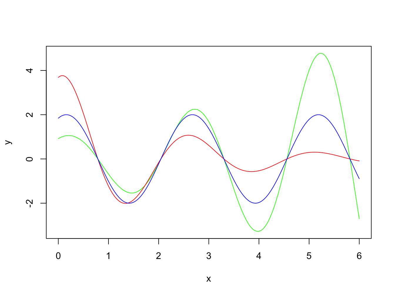
Figure 5.1: $y_{CF}$ for $d > 0$ (red), $d < 0$ (green) and $d = 0$ (blue); all three solutions have the same phase but for clarity of visualisation different amplitudes ($A$) are used in each case.

Example 5.4 Find the general solution of $$\mathcal{L}[y] = \frac{d^2y}{dx^2} - 3 \frac{dy}{dx} + 2y = e^{8x}.$$

• First step: The characteristic equation is $\lambda^2 - 3\lambda + 2 = 0$, so we have $\lambda_1 = 2$ and $\lambda_2 = 1$, so $$y_{CF} = c_1 e^{2x} + c_2 e^x.$$

• Second step: we try ansatz $y_{PI} = A e^{8x}$. $$\mathcal{L}[y_{PI}] = Ae^{8x}[64 - 24 + 2] = e^{8x} \quad \Rightarrow \quad A = \frac{1}{42},$$ So, we have: $$y_{GS} = y_{CF} + y_{PI} = c_1 e^{2x} + c_2 e^x + \frac{1}{42}e^{8x}.$$

Example 5.5 Find the general solution of $$\mathcal{L}[y] = \frac{d^2y}{dx^2} +4 \frac{dy}{dx} + 4y = e^{-2x}.$$

• First step: This case has a charecteristic equation with repeated root $\lambda = -2$, so we have $$y_{CF} = c_1 e^{-2x} + c_2 xe^{-2x}.$$

• Second step: Finding a particular integral $\mathcal{L}[y_{PI}] = f(x).$ 1st try ansatz $y_{PI} = Ae^{-2x}$, which does not work. 2nd try ansatz $y_{PI} = Ax e^{-2x}$, which also does not work. Let’s try ansatz: $y_{PI} = A(x) e^{-2x}$ using the method of variation of parameters. By plugging into the ODE we obtain: $$\frac{d^2A}{dx^2} = 1 \quad \Rightarrow \quad A = \frac{x^2}{2} + B_1x + B_2.$$ So, we obtain the general solution: $$y_{GS} = y_{CF} + y_{PI}= c_1 e^{-2x} + c_2 xe^{-2x} + \frac{x^2}{2}e^{-2x}.$$ Instead of using the method of variation of parameters, we could have guessed the ansatz $y_{PI} = Bx^2 e^{-2x}$ directly and obtaining value of $B$ using the method of undetermined coefficients.

Example 5.6 Find the general solution of $$\mathcal{L}[y] = \frac{d^2y}{dx^2} -2 \frac{dy}{dx} + 2y = e^{x}\sin(x)$$

• First step: Solving the Homogeneous problem $\mathcal{L}[y^H] = 0$. In this case roots are complex, so we have: $$y_{CF} = c_1 e^{(1+i)x} + c_2 e^{(1-i)x}.$$
• Second step: Finding a particular integral $\mathcal{L}[y_{PI}] = f(x).$

Here $f(x)$ can be written as the sum of two functions $$f(x) = e^x\sin{x} = \frac{e^{(1+i)x}}{2i} - \frac{e^{(1-i)x}}{2i}.$$ So, we can use the following two ansatz to find particular integrals using the method of undetermined coefficients: $y^1_{PI} = Ax e^{(1+i)x}$ and $y^2_{PI} = Ax e^{(1-i)x}$. By plugging into the ODE using the first and second part of $f(x)$, one finds values for $A$ and $B$ respectively (left as an exercise for you)  Then the general solution is: $$y_{GS} = y_{CF} + y^1_{PI} + y^2_{PI}.$$

5.4 $k$th order Linear ODEs with constant coefficients

$$\mathcal{L}[y] = \sum_{i=0}^{k} \alpha_i \mathcal{D}^i[y] = f(x); \quad \alpha_i \in \mathbb{R}$$ $$y_{GS}(x; c_1, \cdots, c_k) = y_{CF} + y_{PI} = y^H_{GS}(x; c_1, \cdots, c_k) + y_{PI}(x)$$ First step: Solving the Homogeneous problem $\mathcal{L}[y^H] = 0$

We can try the ansatz $y^H = e^{\lambda x}$: $$\mathcal{L}[e^{\lambda x}] = e^{\lambda x}\sum_{i=0}^{k} \alpha_i \lambda^i = 0 \quad \Rightarrow \quad \sum_{i=0}^{k} \alpha_i \lambda^i = 0.$$ This is the characterstic equation of the $k$th order linear ODE. It has $k$ roots that can be always obtained numerically (in the absence of an analytical solution).

• Case 1: $k$ roots of the characteristic polynomial are distinct:

The solutions $B = \{e^{\lambda_i x}\}_{i=1}^k$ can be shown to be linearly independent using the Wronskian:

$$\mathbb{W}(x) = \begin{bmatrix} e^{\lambda_1 x} & e^{\lambda_2x} & \cdots & e^{\lambda_k x} \\ \lambda_1 e^{\lambda_1 x} & \lambda_2 e^{\lambda_2x} & \cdots & \lambda_k e^{\lambda_k x} \\ \vdots & \vdots & & \vdots \\ & & & \\ \lambda_1^{k-1} e^{\lambda_1 x} & \lambda_2^{k-1} e^{\lambda_2x} & \cdots & \lambda_k^{k-1} e^{\lambda_k x} \end{bmatrix}$$

$$W(x) = \text{det} \, \mathbb{W} (x) = e^{\sum_{i=1}^k \lambda_i x} \begin{vmatrix} 1 & 1 & \cdots & 1 \\ \lambda_1 & \lambda_2 & \cdots & \lambda_k \\ \vdots & \vdots & & \vdots \\ & & & \\ \lambda_1^{k-1} & \lambda_2^{k-1} & \cdots & \lambda_k^{k-1} \, \end{vmatrix} =$$

$$e^{\sum_{i=1}^k \lambda_i x} \prod_{1\leq i < j \leq k} \left( \lambda_i - \lambda_j \right) \neq 0; \quad (\text{Vandermonde determinant})$$ The determinant of the Vandermonde matrix (the matrix obtained above) is a well known result in linear algebra and can be proven using induction. $$B = \{e^{\lambda_1x}, e^{\lambda_2x}, \cdots, e^{\lambda_k x}\} \quad \Rightarrow \quad y_{CF} = \sum_{i=1}^k c_i e^{\lambda_i x}.$$

• Case 2: Not all of the $k$ roots are distinct. Below, we consider the particular case of having $d$ repeated roots and $k-d$ distinct roots.
  $$B = \{e^{\lambda_1x}, e^{\lambda_2x}, \cdots, e^{\lambda_r x}, xe^{\lambda_r x}, \cdots, x^{d-1}e^{\lambda_r x}, e^{\lambda_{r+1} x}, \cdots, e^{\lambda_{k-d+1}x}\} \quad \Rightarrow$$ $$y_{CF} = c_1e^{\lambda_1x}, c_2e^{\lambda_2x}, \cdots, c_re^{\lambda_r x}, c_{r+1}xe^{\lambda_r x}, \cdots, c_{r+d-1}x^{d-1}e^{\lambda_r x}, c_{r+d}e^{\lambda_{r+1} x}, \cdots, c_ke^{\lambda_{k-d + 1}x}.$$

Second step: Finding a particular integral for example for: $\mathcal{L}[y_{PI}] = e^{bx}$, for the case 2 above, we use the following ansatz, using the method of undetermined coefficients:

• if $b \ne \lambda_i$ for $\forall i$ then $y_{PI} = A e^{bx}$.

• if $b = \lambda_i$ for $i \ne r$ then $y_{PI} = Ax e^{bx}$.

• if $b = \lambda_r$ then $y_{PI} = Ax^d e^{bx}$.

5.5 Euler-Cauchy equation

A (rare) example of a linear ODE with non-constant coefficients that we can solve analytically is the Euler-Cauchy ODE: $$\mathcal{L}[y] = \beta_k x^k \frac{d^ky}{dx^k} + \beta_{k-1} x^{k-1} \frac{d^{k-1}y}{dx^{k-1}} + \cdots + \beta_1 x \frac{dy}{dx} + \beta_0 y = f(x).$$ Using the change of variable $x = e^z$, the Euler-Cauchy equation can be transformed into a linear ODE with constant coefficients.

Example 5.7 Solve the following ODE: $x^2 \frac{d^2y}{dx^2} + 3 x \frac{dy}{dx} + y = x^3$.

Using the change of variable $x = e^z$ we have $z = \ln{x}$ and so: $$\frac{dy}{dx} = \frac{dy}{dz} \frac{dz}{dx} = \frac{1}{x}\frac{dy}{dz} \quad \Rightarrow \quad x\frac{dy}{dx} = \frac{dy}{dz},$$

$$\frac{d^2y}{dx^2} = \frac{d}{dx}\left( \frac{dy}{dx} \right) = \frac{d}{dz}\left( \frac{dy}{dx} \right) \frac{dz}{dx} = \frac{1}{x^2}\left[\frac{d^2y}{dz^2} - \frac{dy}{dz}\right].$$ So, in terms of the new independent variable we have the following linear ODE with constant coefficients.
$$\frac{d^2y}{dz^2} + 2 \frac{dy}{dz} + y = e^{3z}.$$ By obtaining the complementary function and particular integral, we have the following general solution: $$y_{GS}(z; c_1, c_2) = y_{CF} + y_{PI} = c_1 e^{-z} + c_2 z e^{-z} + \frac{1}{16} e^{3z}.$$ So, in the general solution in terms of $x$ is: $$y_{GS}(x; c_1, c_2) = \frac{c_1}{x} + c_2\frac{\ln{x}}{x} + \frac{1}{16}x^3.$$

5.6 Using Fourier Transforms to solve linear ODEs

As Fourier transform is a linear operation, and given the properties we had for Fourier transforms of derivatives of a function seen in Section 2.1, one can use Fourier transforms to solve linear ODEs or find particular integrals. This is particularly relevant for solving partial differential equations as discussed in the second year. Here we discuss an example.

Example 5.8 Find a solution for the following ODE, known as the Airy equation or the Stokes equation, which arises in different areas of physics. Assume $\lim_{x \rightarrow \pm \infty} y(x) = 0$. $$\frac{d^2y}{dx^2} - x y = 0.$$

This is a linear 2nd order ODE with non-constant coefficients and so far we have not seen a method of solving it. Note that this ODE is not also one of the types that are discussed in Section 4.2. Our strategy is to take Fourier transform from this ODE and see if we can solve for the Fourier transform. Using the properties in Section 2.1, we obtain: $$-\omega^2 \hat{y}(\omega) -i\frac{d\hat{y}(\omega)}{d\omega} = 0$$
This is a first order ODE for $\hat{y}(\omega)$, by solving it we obtain: $$\hat{y}(\omega) = c e^{\frac{i\omega^3}{3}},$$ where $c$ is an arbitrary constant of integration. Using the inverse transform we obtain: $$y(x) = \frac{c}{2\pi} \int^\infty_{-\infty} e^{i(\omega x + \omega^3/3)} \,d\omega = \frac{c}{\pi}\int^\infty_{0} \cos(\omega x + \frac{\omega^3}{3})\,d\omega,$$ where, in the last step we have used the evenness of cosine and oddness of the sine function. For $c = 1$ the function $y(x)$ is known as the Airy function (of the first kind) and is denoted by $Ai(x)$. It is defined as the above integral and cannot be reduced further and is a solution of the Airy ODE.