6 Tutorial 6: Control structures & functions in R

After working through Tutorial 6, you’ll…

• understand how to write your own control structures
• understand how to write your own functions

Data

For this tutorial, we’ll use a new data set “data_tutorial6.txt” (via OLAT/Materials/Data for R).

The data set consists of data that is completely made up - a survey with 1000 citizens in Europe.

The data file “data_tutorial6.txt” is structured as follows:

• Each row contains the answer for a single citizen.
• Each column contains all values given by citizens for a single variable.

The five variables included here are:

• country: the country in which each citizen was living at the time of the survey (France/Germany/Italy/Switzerland)
• date: the date on which each citizen was surveyed (from 2021-09-20 to 2021-10-03)
• gender: each citizen’s gender (female/male/NA)
• trust_politics: how much each citizen trusts the political system (from 1 = no trust at all to 4 = a lot of trust)
• trust_news_media: how much each citizen trusts the news media (from 1 = no trust at all to 4 = a lot of trust)

Read in the data set:

data <- read.csv2("data_tutorial 6.txt")

This is how the data looks like in R:

head(data)

##       country       date gender trust_politics trust_news_media
## 1     Germany 2021-09-20 female              3                1
## 2 Switzerland 2021-10-02   male              2                1
## 3      France 2021-09-21   <NA>              1                3
## 4       Italy 2021-10-03   male              2                2
## 5     Germany 2021-09-21 female              3                1
## 6 Switzerland 2021-09-20   male              1                2

6.1 Control structures

What are control structures?

Sometimes, you may want R to not execute all of your code but only chunks of it.

To control the flow of the program, especially which chunks of code should be run or how often/for which objects code should be run, we can use so-called control structures, including:

• if/else conditions: R executes functions only if specific conditions are fulfilled.
• loops: We often need R to execute functions in an iterative way, i.e., repeatedly apply the same function to different objects

6.1.1 if/else conditions

If/else conditions are helpful for running code only if specific conditions are fulfilled (and specifying which other functions should be executed else). In if/else conditions, you have to specify at least one if condition (or several), while the command for which code should executed otherwise (i.e., else) is obligatory.

Image: if/else conditions

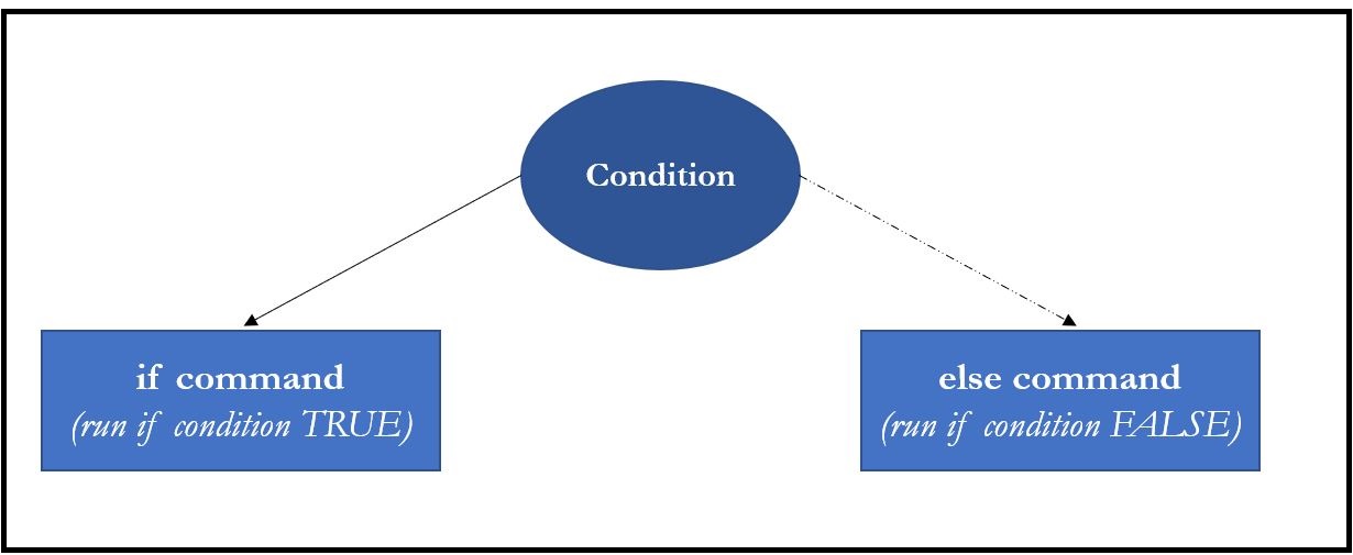
if(condition){
  # function that should be executed
  # if condition true
} else{
  # function that should be executed
  # if condition not true
}

Let’s start with an example: You want to check whether the variable date has been imported in character or another format and for R to tell you which format is correct.

In short:

• if the variable date is saved in character format, R should print: “Variable is saved in character format”
• else, R should print: “Variable is saved in a different format”

In code, this would look something like this:

First if condition:

if(is.character(data$date) == TRUE){
  print("Variable is saved in character format")
}

## [1] "Variable is saved in character format"

Here, R prints out the sentence “Variable is saved in character format” because the variable is indeed saved in character format (and, thus, the condition is TRUE).

If/else condition

Let’s bring this condition together with the else command telling R what do to if the if command is not true.

if(is.character(data$date) == TRUE){
  print("Variable is saved in character format")
} else {
  print("Variable is saved in a different format")
}

## [1] "Variable is saved in character format"

Bringing these functions together, we see that only the first condition - the variable date being saved in character format - is true. Thus, only the first block of code is run while the else command is ignored.

If we run the same command with variables we know to be saved in non-character format - for instance the variable trust_politics, we get a different result (since the if condition is not true and, thus, the code after else is run):

if(is.character(data$trust_politics) == TRUE){
  print("Variable is saved in character format")
} else {
  print("Variable is saved in a different format")
}

## [1] "Variable is saved in a different format"

While you may not use if/else conditions very often, they are sometimes useful - for instance, if you want to write your own functions and want to print error messages based on specific conditions.

Another example - we discussed this in the seminar, so I’m adding this due to popular demand :).

The following if/else condition will only print one of the two statements:

if((1 > 2) == TRUE){
  print("1 is bigger than 2")
} else {
  print("1 is smaller than 2")
}

## [1] "1 is smaller than 2"

What is the reason for that?

Since the first if condition - 1 > 2 - is not true, the if condition is ignored. Instead, R executes the code related to the else condition.

6.1.2 Loops

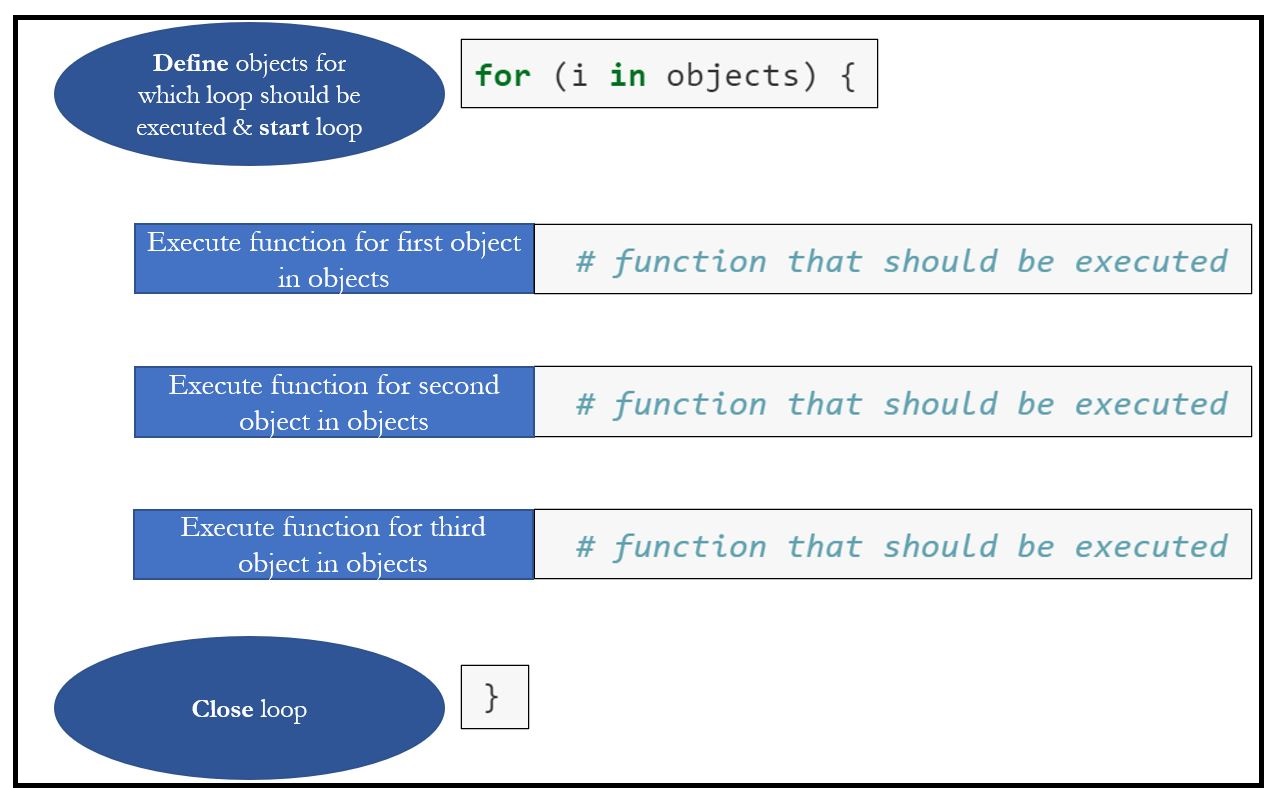
In R, you may often have to execute functions in an iterative way, i.e., repeatedly apply the same function to different objects. For loops do just that.

This is how for loops look like:

for (i in objects) {
  # function that should be executed
}

What does this for loop indicate?

• The first row describes for which object i in a sequence of objects objects a command should be executed. The loop takes every unique object i out of objects.
• It then applies the subsequent function defined between the curly brackets {} to this object i.

In short: For every object i in objects, the function between the curly brackets would be executed.

Image: Loop

An easy example: We may want R to print the country from which a surveyed citizen comes - but only for every 100st citizen in the survey.

We could do this with code in a form that we already know:

data$country[100]

## [1] "Italy"

data$country[200]

## [1] "Italy"

data$country[300]

## [1] "Italy"

data$country[400]

## [1] "Italy"

#and so on

Or we use a for loop which does the same, but with fewer lines of code.

We tell R to take every object i in the vector c(100,200,300,400,500,600,700,800,900,1000) and print the corresponding country:

for (i in c(100,200,300,400,500,600,700,800,900,1000)) {
 print(data$country[i])
}

## [1] "Italy"
## [1] "Italy"
## [1] "Italy"
## [1] "Italy"
## [1] "Italy"
## [1] "Italy"
## [1] "Italy"
## [1] "Italy"
## [1] "Italy"
## [1] "Italy"

Take another example: The following loop takes every single number i out of the sequence of numbers 1:10. R then prints all these numbers - i.e., every i in 1:10.

for (i in 1:10){
  print(i)
}

## [1] 1
## [1] 2
## [1] 3
## [1] 4
## [1] 5
## [1] 6
## [1] 7
## [1] 8
## [1] 9
## [1] 10

Later on, you will mostly use objects defined outside of the loop, for instance like so:

numbers <- 1:10
for (i in numbers){
  print(i)
}

## [1] 1
## [1] 2
## [1] 3
## [1] 4
## [1] 5
## [1] 6
## [1] 7
## [1] 8
## [1] 9
## [1] 10

Wow - feels like we have advanced to hacker-levels already!

In fact, this is exactly the same as the loop before - we have just defined our objects numbers outside of the loop, which makes the loop look much more abstract.

You won’t use loops in too many cases (and better alternative such as the purrr package belonging to the tidyverse exist). However, it is useful to understand how they work - which is why you should know about their general structure.

6.2 Custom functions

In some case, the function you need may simply not (yet) exist. In this case, you have to write your own custom functions.

For this, it is important to know how functions work.

For example, how is the mean() function structured? To get the function’s source code, you can use the following command. We have to look for the mean.default function for technical reasons - I won’t go into details here and you don’t need to know why this is the case, but if you are interested see this discussion.

getAnywhere(mean.default)

## A single object matching 'mean.default' was found
## It was found in the following places
##   package:base
##   registered S3 method for mean from namespace base
##   namespace:base
## with value
## 
## function (x, trim = 0, na.rm = FALSE, ...) 
## {
##     if (!is.numeric(x) && !is.complex(x) && !is.logical(x)) {
##         warning("argument is not numeric or logical: returning NA")
##         return(NA_real_)
##     }
##     if (na.rm) 
##         x <- x[!is.na(x)]
##     if (!is.numeric(trim) || length(trim) != 1L) 
##         stop("'trim' must be numeric of length one")
##     n <- length(x)
##     if (trim > 0 && n) {
##         if (is.complex(x)) 
##             stop("trimmed means are not defined for complex data")
##         if (anyNA(x)) 
##             return(NA_real_)
##         if (trim >= 0.5) 
##             return(stats::median(x, na.rm = FALSE))
##         lo <- floor(n * trim) + 1
##         hi <- n + 1 - lo
##         x <- sort.int(x, partial = unique(c(lo, hi)))[lo:hi]
##     }
##     .Internal(mean(x))
## }
## <bytecode: 0x0000020120ebfa30>
## <environment: namespace:base>

Wow, that looks complicated. But is it?

In short, the source code includes the following main three elements:

function_name <- function(argument_1, argument_2){
  #Code to be executed, including which results the function should return
  return()
}

Elements of functions:

• the function’s name (here, mean)
• the function’s arguments (here, x as a necessary argument that needs to be specified and trim or na.rm as arguments that can be specified but are otherwise set to predefined default values)
• the function’s code (here a range of rules for how the mean of different objects should be computed and which result should be returned with return()

Let’s take an example: We may have a vector numbers consisting of a sequence of numbers from 1 to 100:

numbers <- c(1:100)

If we wanted to calculate the mean of this vector, we could simply call the function mean():

mean(numbers)

## [1] 50.5

However, we could also write our own function called mean_new like so:

mean_new <- function (x) 
{
  n <- length(x)
  sum <- sum(x)
  result <- sum/n
  return(result)
}

What does this code do?

1. First, we specify the name of the new function: mean_new
2. Second, we specify which arguments the function should consider: here, x as the object of which the mean should be computed.
3. Third, inside the curly brackets {}, we specify how the function should work:
   • We count the number of unique elements inside the vector number: n
   • We take the sum of the values inside the vector number: sum
   • We calculate the mean: result
   • We advise the function to only return the object result when applying the function (not the objects n or sum)

When executing the code, you will see that R saved the new function mean_new() as a new object in your working space. Let’s try if it works!

mean_new(numbers)

## [1] 50.5

Looks good - R only returns the result of our calculations (note that neither the objects n nor sum will turn up in your working environment).

6.3 Take Aways

• if/else conditions: allow you to execute chunks of code only if specific conditions are fulfilled
• loops: allow you to execute code repeatedly, i.e., apply the same function to different objects
• functions: are what keeps R alive. You can use functions already existing in R, load new functions via packages, or create your own functions.

6.4 More tutorials on this

You still have questions? The following tutorials & papers can help you with that:

• R for Data science by G. Grolemund and H. Wickham, Tutorial 19 and 21
• R Codebook by J.D. Long and P. Teetor, Tutorial 15
• YaRrr! The Pirate’s Guide to R by N.D.Phillips, Tutorial 16 and 17
• R Codebook, 2nd Edition by James Long and Paul Teetor, Tutorial 15

6.5 Test your knowledge

You’ve worked through all the material of Tutorial 6? Let’s see it - the following tasks will test your knowledge.

Import the same data as used in the tutorial, the new data set “data_tutorial6.txt” (via OLAT/Materials/Data for R).

Remember, the five variables included here are:

• country: the country in which each citizen was living at the time of the survey (France/Germany/Italy/Switzerland)
• date: the date on which each citizen was surveyed (from 2021-09-20 to 2021-10-03)
• gender: each citizen’s gender (female/male/NA)
• trust_politics: how much each citizen trusts the political system (from 1 = no trust at all to 4 = a lot of trust)
• trust_news_media: how much each citizen trusts the news media (from 1 = no trust at all to 4 = a lot of trust)

6.5.1 Task 6.1

Writing the corresponding R code,

• add the value of the previous observation in the data set to every value belonging to the variable trust_politics. Save the resulting vector in a variable called trust_politics_new.

In this case, the first observation should be coded as NA. The second observation should include the sum of the first and the second observation, the third observation should include the values of the second and third observation, etc.

The result should then look something like this (see the old values on the left and the new values on the right):

head(data[c("trust_politics", "trust_politics_new")])

##   trust_politics trust_politics_new
## 1              3                 NA
## 2              2                  5
## 3              1                  3
## 4              2                  3
## 5              3                  5
## 6              1                  4

Thus:

• the first row is set to NA.
• the second row contains the sum of the first and second observation (3 + 2 = 5).
• the third row contains the sum of the second and third observation (2 + 1 = 3).
• etc.

6.5.2 Task 6.2

Writing the corresponding R code,

• create a new function called stupid_sum()
• the function should have two arguments that need to be filled: a vector x and a vector y
• the function should print the sum of both vectors if both vectors include numeric data.
• the function should print the error “I simply can’t” if any of the two vectors include any type of non-numeric data.

Important: This is a tricky task - so if you can’t do parts of it, don’t be frustrated. Just try to get as far as you can.

The result should then look something like this when testing it with a range of numeric/non-numeric vectors:

#When testing the function
stupid_sum(x = data$trust_politics, y = data$trust_news_media)

## [1] 5010

stupid_sum(x = data$trust_politics, y = data$country)

## [1] "I simply can't"

This is where you’ll find solutions for tutorial 6.

Let’s keep going: Tutorial 7: Descriptive statistics