12 Tutorial 12: Rule-based approaches & dictionaries
In Tutorial 12, you will learn about rule-based approaches & dictionaries, especially
- How to get general descriptive statistics on your corpus
- How to apply rule-based approaches (especially keywords-in-context & co-occurrence analysis)
- How to conduct dictionary analysis
Let’s use the same data as in the previous tutorials. You can find the corresponding R file in OLAT (via: Materials / Data for R) with the name immigration_news.rda.
Source of the data set: Nulty, P. & Poletti, M. (2014). “The Immigration Issue in the UK in the 2014 EU Elections: Text Mining the Public Debate.” Presentation at LSE Text Mining Conference 2014. Accessed via the quanteda corpus package.
load("immigration_news.rda")By applying some of the preprocessing steps in the last tutorial, we prepare the corpus for analysis:
- We save the publication month of each text (we’ll later use this vector as a document level variable)
- We remove the pattern for a line break \n.
- We tokenize our texts, remove punctuation/numbers/URLs, transform the corpus to lowercase, and remove stopwords.
- We apply relative pruning
- We save the result as a document-feature-matrix called dfm
library("stringr")
library("quanteda")

#extracting the publication month
data$month <- str_extract(string = data$text, pattern = "[0-9]+ (january|february|march|april|may|june|july|august|september|october|november|december) 2014")
data$month <- str_extract(string = data$month, pattern = "january|february|march|april|may|june|july| august|september|october|november|december")

#turning the publication month into a numeric format
data$month[data$month=="february"] <- "2"
data$month[data$month=="march"] <- "3"
data$month[data$month=="april"] <- "4"
data$month[data$month=="may"] <- "5"

#removing the pattern indicating a line break
data$text <- gsub(pattern = "\n", replacement = " ", x = data$text)

#tokenization & removing punctuation/numbers/URLs etc.
tokens <- data$text %>%
          tokens(what = "word",
                 remove_punct = TRUE,
                 remove_numbers = TRUE,
                 remove_url = TRUE) %>%
          tokens_tolower() %>%
          tokens_remove(stopwords("english"))

#applying relative pruning
dfm <- dfm_trim(dfm(tokens), min_docfreq = 0.005, max_docfreq = 0.99,
                docfreq_type = "prop", verbose = TRUE)
## Removing features occurring:## - in fewer than 14.165 documents: 33,992## - in more than 2804.67 documents: 2## Total features removed: 33,994 (86.8%).#This is our dfm
dfm## Document-feature matrix of: 2,833 documents, 5,162 features (97.14% sparse) and 0 docvars.
## features
## docs support ukip continues grow labour heartlands miliband scared leo mckinstry
## text1 2 7 1 1 8 2 4 1 1 1
## text2 0 1 0 0 0 0 0 0 0 0
## text3 0 1 0 0 0 0 0 0 0 0
## text4 0 0 0 0 0 0 0 0 0 0
## text5 0 1 0 0 0 0 0 0 0 0
## text6 0 0 0 0 0 0 0 0 0 0
## [ reached max_ndoc ... 2,827 more documents, reached max_nfeat ... 5,152 more features ]12.1 Descriptive statistics
12.1.1 Number of documents
First, you may want to know how many documents the corpus contains. Using the ndoc() command, we see: about 2,800 articles.
ndoc(dfm)## [1] 283312.1.2 Number of features
Next, we may want to know how many features our corpus contains. As you can see, even after preprocessing, our corpus still contains more than 5,000 features.8
nfeat(dfm)## [1] 516212.1.3 Feature Occurrence
Now, we may want to know how often each feature occurs. Using the featfreq() command, we do exactly that:
features <- as.data.frame(featfreq(dfm))The names of each feature is now saved as the corresponding row name, but not as a separate variable. This command changes that:
features$feature <- rownames(features)
colnames(features) <- c("freq", "feature")
features[1:10,]
## freq feature
## support 716 support
## ukip 3606 ukip
## continues 60 continues
## grow 72 grow
## labour 2144 labour
## heartlands 29 heartlands
## miliband 580 miliband
## scared 57 scared
## leo 29 leo
## mckinstry 20 mckinstryUsing these commands, we can for instance see how often a specific feature - for example, the feature crisis - is used across the corpus:
features$freq[features$feature=="crisis"]## [1] 22812.1.4 Frequent & rare features
Next, we may want to know which features are most or least frequent.
We first display the 20 most frequent features…
topfeatures(dfm, 20)## said mr ukip immigration people party one uk britain farage
## 5513 3779 3606 3533 3386 2821 2644 2511 2395 2329
## rights eu may labour © reserved news british last telegraph
## 2326 2324 2183 2144 2090 1979 1970 1900 1899 1830… followed by the 10 least frequent features
topfeatures(dfm, decreasing = FALSE, 20)## giles reminds successive bureaucrats enduring alarm dire stating contender pursuit
## 15 15 15 15 15 15 15 15 15 15
## hinted swiftly indicator backfired onslaught shore veterans extensive avoided uncertain
## 15 15 15 15 15 15 15 15 15 1512.1.5 Visualizing feature occurrences
A popular (but among many scientists now rather frowned upon) trend is to visualize frequent words with wordclouds.
Using the wordcloud() function, we visualize feature frequencies - the larger features displayed here, the more frequently they occur in our corpus.
To use the package, you need to install and activate the quanteda.textplots package.
Here, we visualize the most frequent 50 words:
library("quanteda.textplots")
textplot_wordcloud(dfm, max_words = 50, color = "grey10")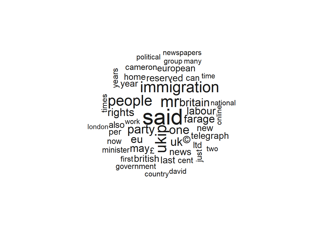
From the wordcloud, we can at least learn some things about our texts - namely that they are in English and deal with British politics and/or immigration.
12.2 Grouped feature occurrences
Let’s say that we want to know how the occurrence of features differs across months, i.e. we want to depict trends.
To do this, we first use and set the publication month of each article as a grouping variable, i.e., the variable based on which we want to compare the frequency of a pattern.
dfm$month <- as.numeric(data$month)Next, we use dfm_group() to create a grouped document_feature_matrix called dfm_group.
Note that we only have four rows in this dfm since we only have four groups (the months February, March, April, & May) in our data set.
dfm_group <- dfm_group(dfm, groups = month)
dfm_group
## Document-feature matrix of: 4 documents, 5,162 features (4.42% sparse) and 1 docvar.
## features
## docs support ukip continues grow labour heartlands miliband scared leo mckinstry
## 2 72 125 6 3 113 2 37 3 3 2
## 3 239 898 20 23 667 6 140 11 15 9
## 4 231 1115 20 26 635 12 151 21 9 7
## 5 174 1468 14 20 729 9 252 22 2 2
## [ reached max_nfeat ... 5,152 more features ]Next, we use the textstat_frequency() command to receive information about both the absolute and the relative frequency with which a feature occurs.
- the absolute number tells us how often each feature occurs each month
- the relative number tells us which share of all feature occurrences each feature takes up each month. This normalizes, for instance, for the fact that we may simply have more articles being published in some months compared to others, which increases the overall amount with which features are prevalent for those months with more overall texts.
To use the function, you need to install and activate the quanteda.textstats package.
library("quanteda.textstats")
freq <- textstat_frequency(dfm_group, group = month)
freq[1:10]
## feature frequency rank docfreq group
## 1 said 462 1 1 2
## 2 immigration 362 2 1 2
## 3 mr 332 3 1 2
## 4 eu 324 4 1 2
## 5 britain 294 5 1 2
## 6 people 277 6 1 2
## 7 uk 271 7 1 2
## 8 february 262 8 1 2
## 9 year 251 9 1 2
## 10 £ 226 10 1 2We may want to know whether certain features occurred more or less frequently over time.
For example, we are interested in whether the word immigration occurred more or less frequently in our corpus over time.
To do this, we focus on this feature:
freq_immigration <- freq[freq$feature=="immigration"]
freq_immigration
## feature frequency rank docfreq group
## 2 immigration 362 2 1 2
## 4382 immigration 1475 2 1 3
## 9506 immigration 837 7 1 4
## 14627 immigration 859 8 1 5Next, we use our knowledge from Tutorial 8: Visualizing data to visualize the occurrence of the feature immigration over time:
library("ggplot2")
ggplot(freq_immigration, aes(x = group, y = frequency, group = 1)) +
  geom_line(size = 1, color = "darkgreen") +
  scale_x_discrete("Month", labels = c("February", "March", "April", "May")) +
  labs(y = "N (Feature Immigration)",
       title = "Absolute occurrence of the feature immigration over time") +
  theme_light()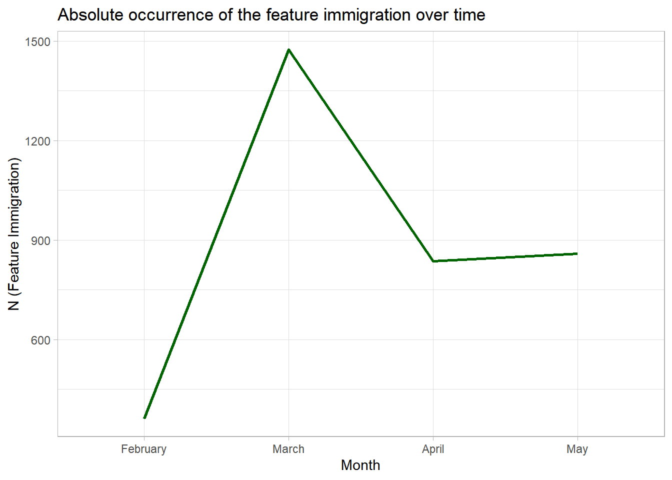
The plot indicates that the feature immigration occurred more frequently in some months than in others.
However, we should be careful in interpreting absolute feature occurrences.
By only considering this graph, we might for example think that the feature immigration was mentioned far more often in March.
However, the low frequency of the word may be partly due to the fact that our corpus includes slightly more texts from March (at least compared to February), thereby increasing the overall occurrence of the feature immigration in this month:
table(data$month)##
## 2 3 4 5
## 252 933 835 813Quanteda also allows you to calculate the relative percentage with which a feature occurs (in comparison to all other features) via the dfm_weight() function. I would advise you to rely on relative feature occurrences, especially if your groups differ in sample size or lengths of texts.
Let’s therefore consider the relative occurrence of a feature, i.e., the overall % of feature occurrences belonging to the feature immigration in comparison to all other features (indicating how often the feature was mentioned compared to all other feature occurrences in the same month):
dfm_group_relative <- dfm_weight(dfm_group, scheme = "prop")
freq <- textstat_frequency(dfm_group_relative, group = month)
freq[1:10]
## feature frequency rank docfreq group
## 1 said 0.009393681 1 1 2
## 2 immigration 0.007360416 2 1 2
## 3 mr 0.006750437 3 1 2
## 4 eu 0.006587776 4 1 2
## 5 britain 0.005977797 5 1 2
## 6 people 0.005632142 6 1 2
## 7 uk 0.005510146 7 1 2
## 8 february 0.005327152 8 1 2
## 9 year 0.005103493 9 1 2
## 10 £ 0.004595177 10 1 2We again visualize our results:
freq_immigration <- freq[freq$feature=="immigration"]

ggplot(freq_immigration, aes(x = group, y = frequency, group = 1)) +
  geom_line(size = 1, color = "darkgreen") +
  scale_x_discrete("Monat", labels = c("February", "March", "April", "May"))+
  labs(y = "Occurrence of the feature immigration (in %, compared to all other features)",
       title = "Relative occurrence of the feature immigration over time")+
  theme_light()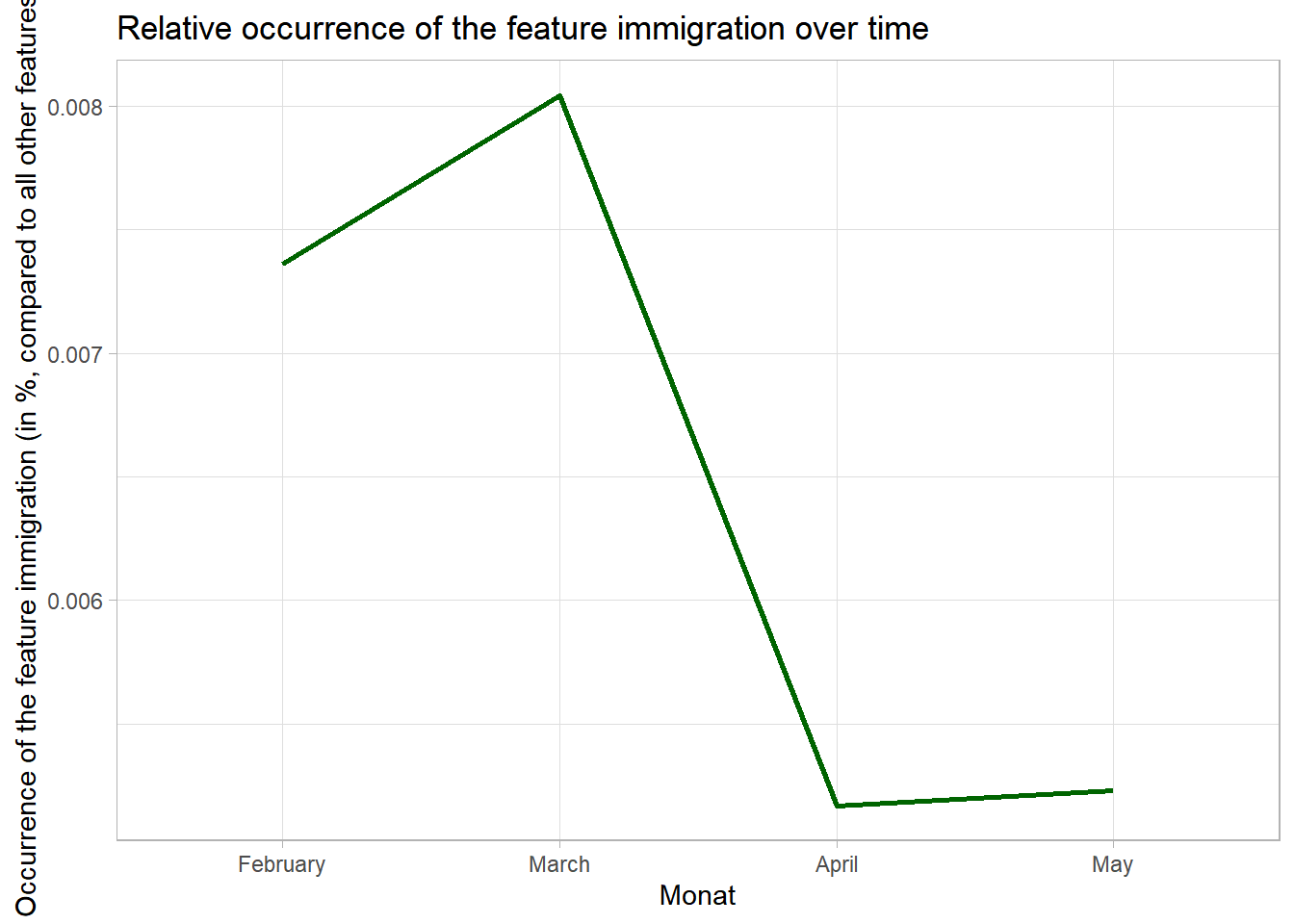
12.3 Rule-based approaches
In the following, I’ll introduce you to two rule-based approaches to analyze texts:
- keywords-in-context
- co-occurrence analysis
12.3.1 Keywords-in-context
In class, I’ve tried to make you aware about the many (false) assumptions we rely on when using bag-of-words approaches. This includes the fact that we assume that we can ignore the order and context of words to understand texts.
Oftentimes, doing so may be problematic - especially if we, for instance, want to know how entities are talked about (i.e., consider entity-specific sentiment).
Suppose we want to know whether the word immigration is more likely to be described with negative or with more positive words in our corpus.
To analyze this, we may want to know whether words used in close distance to the feature immigration are negative or positive (since this would be very indicative for immigration being describe in a positive or negative light).
To answer this question, we can do a keywords-in-context analysis.
Keywords-in-context describes a method where we search for a certain keyword - for example immigration - and retrieve words before or after this keyword.
Suppose we want to find any three features before and after the keyword immigration to get a better sense of words used to describe immigration.
The kwic() command gives us all n words before and after a pattern in the text string x.
kwic <- kwic(tokens(data$text), pattern =  "immigration", window = 3)
head(kwic, 10)
## Keyword-in-context with 10 matches.
## [text1, 371] obsessed with mass | immigration | multi-cultural diversity european
## [text2, 132] britains broken open-door | immigration | policy the disease-ridden
## [text2, 343] past year calais | immigration | chief and deputy
## [text2, 402] seeking to evade | immigration | control they are
## [text3, 130] britains broken open-door | immigration | policy the disease-ridden
## [text3, 353] past year calais | immigration | chief and deputy
## [text5, 157] secure units under | immigration | laws at the
## [text5, 241] with the illegal | immigration | issue itself by
## [text5, 386] and deserve an | immigration | system that is
## [text5, 399] crack down on | immigration | offenders when weWe could use keywords-in-context to see, for example, how immigration is described. Later on, this may be helpful to create our own dictionaries - for example, to find words used to describe immigration in a negative or positive way.
Here, we want to use keywords-in-context for another type of analysis: For example, we could analyze whether the word crime is mentioned around the term immigration, i.e., whether immigration is associated with crime.
Our question: Do newspapers associate immigration with crime?
To do so, we retrieve the three words any text mentions before the pattern immigration, the pattern itself, and the three words after the pattern immigration as a text string. The paste command merges these three variables in the kwic object and saves the result as the vector context_immigration.
context_immigration <- paste(kwic$pre, kwic$keyword, kwic$post)
context_immigration[1:5]
## [1] "obsessed with mass immigration multi-cultural diversity european"
## [2] "britains broken open-door immigration policy the disease-ridden"
## [3] "past year calais immigration chief and deputy"
## [4] "seeking to evade immigration control they are"
## [5] "britains broken open-door immigration policy the disease-ridden"Next, we can simply count how often the word crime appears in the context of the keyword immigration:
sum(str_count(context_immigration, pattern = "crime"))## [1] 5Overall, crime is mentioned no more than five times in the context of immigration - not that much.
12.4 Co-occurrence analysis
Similar to the previous analysis, we may not only want to know whether a word - such as crime - is mentioned in close context to the word immigration. More generally, we may want to know whether texts about immigration also mention crime or other negative terms anywhere - may it be directly related to/in the context of the term immigration or somewhere else in text.
We want to know: Do newspapers often use the patterns immigration and crime in the same text?
To answer this question, we need to look at the co-occurrence of words - that is, whether two words occur together in a text. This does not mean that these words occur directly after each other or even in proximity to each other - only that both are mentioned in the same text.
To do so, we create a co-occurrence matrix which is similar to the document-feature matrix:
- the columns of a co-occurrence matrix denote features
- the rows of a co-occurrence matrix also denote features
- the cells indicate how often a feature occurs together with another feature in texts.
Let’s look at an example.
We first create the co-occurrence matrix:
fcm <- fcm(dfm)
fcm
## Feature co-occurrence matrix of: 5,162 by 5,162 features.
## features
## features support ukip continues grow labour heartlands miliband scared leo mckinstry
## support 330 1850 24 18 1062 37 198 24 14 12
## ukip 0 9754 84 45 5467 164 1427 160 41 40
## continues 0 0 2 3 45 2 13 1 6 5
## grow 0 0 0 5 24 2 12 1 1 1
## labour 0 0 0 0 3689 181 2277 107 37 37
## heartlands 0 0 0 0 0 9 63 4 4 4
## miliband 0 0 0 0 0 0 639 41 11 11
## scared 0 0 0 0 0 0 0 27 1 1
## leo 0 0 0 0 0 0 0 0 5 22
## mckinstry 0 0 0 0 0 0 0 0 0 1
## [ reached max_feat ... 5,152 more features, reached max_nfeat ... 5,152 more features ]Next, we ask R to only focus on specific terms.
Using fcm_select(), we reduce the co-occurrence matrix to a set of selected features: immigration, a set of positive (chance, good), neutral (work, visa), and negative (crime, threat) words.
fcm <- fcm_select(fcm,
                  pattern = c("immigration",
                              "chance", "good",
                              "work", "visa",
                              "crime", "threat"),
                  selection = "keep")
We then visualize the co-occurrence of these features as a network.
Features are connected by lines if they co-occur in the same document. The more often two features occur together, the thicker these lines.
For example, the word immigration co-occurs frequently with work, as you can see from the overall thicker lines connecting both features. Co-occurrences of the feature immigration and crime, in contrast, are less frequent.
textplot_network(fcm)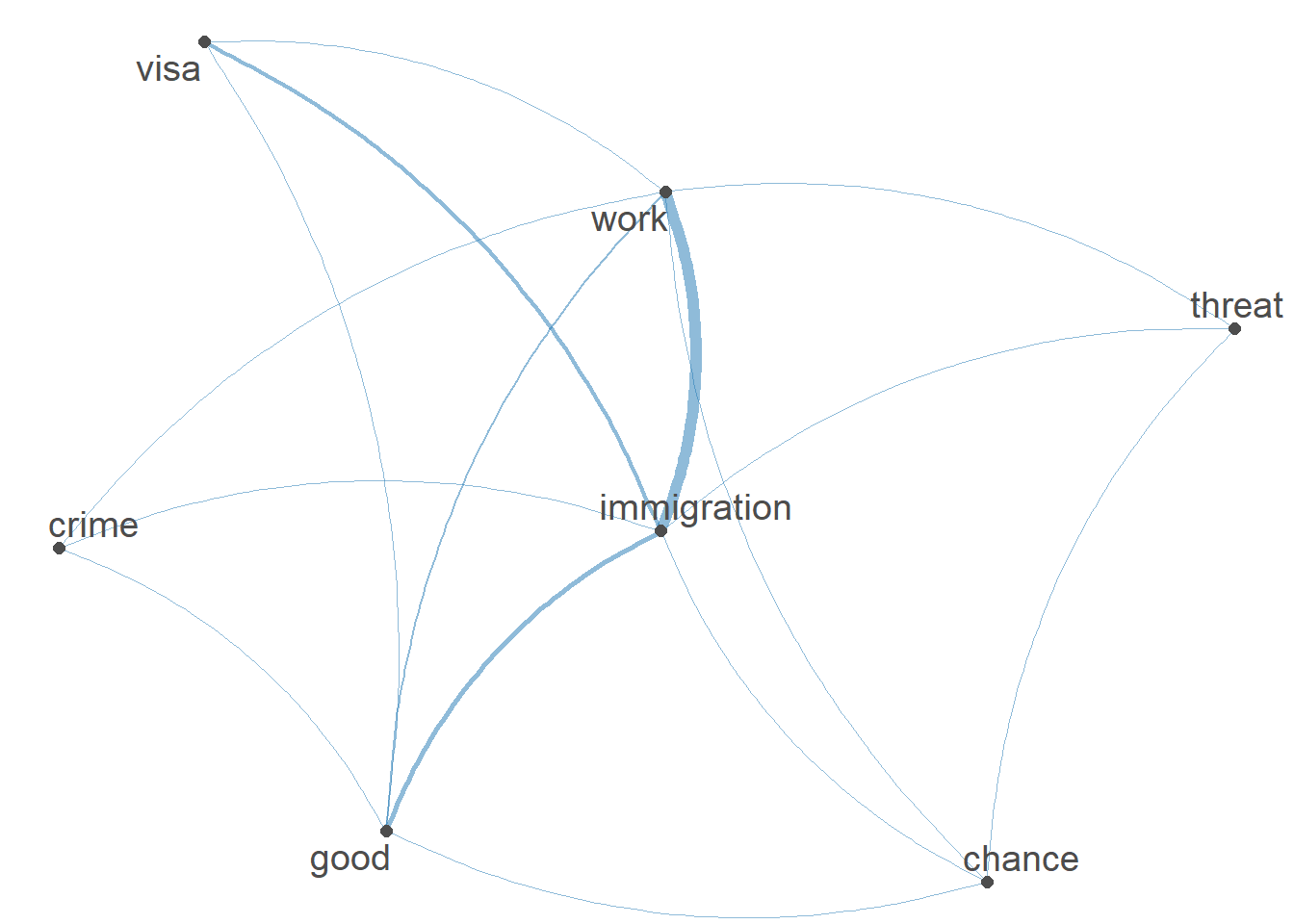
If we don’t want to infer these co-occurrences from the network graph, we can simply inspect the co-occurrence matrix.
To do so, the quanteda package provides the useful convert() function. Quanteda objects, including the co-occurrence matrix used here, can thereby be converted into base R types of objects such as a data frame:
fcm <- convert(fcm, to = "data.frame")
fcm
## doc_id threat immigration work good crime visa chance
## 1 threat 51 237 56 36 19 9 42
## 2 immigration 0 4556 1790 873 198 605 213
## 3 work 0 0 826 359 60 219 77
## 4 good 0 0 0 247 42 147 43
## 5 crime 0 0 0 0 236 20 21
## 6 visa 0 0 0 0 0 273 5
## 7 chance 0 0 0 0 0 0 42Relying on the the dataframe format, we can easily use our knowledge about how to access specific rows and cells in data frames to understand how often exactly these features co-occur.
fcm[fcm$doc_id == "immigration", c("crime")]## [1] 198fcm[fcm$doc_id == "immigration", c("work")]## [1] 179012.5 Dictionary analysis
Let us now turn to a popular method related to automated content analysis: analysis via dictionaries.
Dictionaries are lists of features. Based on the manifest occurrence of certain features - for example, the words “crisis”, “bad” and “devastating” - the occurrence of a latent construct - for example, negative sentiment - is inferred.
In the seminar, we distinguished between two types of dictionaries.
- Off-the-shelf dictionaries as existing word lists, often developed for other types of texts or topics.
- Organic dictionaries as word lists you create manually for your type of text, topic, and the latent construct of interest.
You have already learned the basic logic and problems of dictionary analyses in the seminar. Let’s now do these analyses in R.
12.5.0.1 Off-the-shelf dictionaries
In the seminar, I’ve already talked about the very limited validity of many off-the-shelf dictionaries. Please always keep this in mind when applying such dictionaries. At the very least, you need to validate your results to show readers whether you actually measure what you claim to measure. For further discussions about the issue, see for example Boukes et al., 2020, Chan et al., 2020 oder Stine, 2019.
The quanteda includes, among others, the Lexicoder Sentiment Dictionary including word lists created to capture negative or positive sentiment based on Young & Soroka, 2012a as well as Young & Soroka (2012b): Lexicoder Sentiment Dictionary.
Let’s inspect the dictionary
data_dictionary_LSD2015## Dictionary object with 4 key entries.
## - [negative]:
## - a lie, abandon*, abas*, abattoir*, abdicat*, aberra*, abhor*, abject*, abnormal*, abolish*, abominab*, abominat*, abrasiv*, absent*, abstrus*, absurd*, abus*, accident*, accost*, accursed* [ ... and 2,838 more ]
## - [positive]:
## - ability*, abound*, absolv*, absorbent*, absorption*, abundanc*, abundant*, acced*, accentuat*, accept*, accessib*, acclaim*, acclamation*, accolad*, accommodat*, accomplish*, accord, accordan*, accorded*, accords [ ... and 1,689 more ]
## - [neg_positive]:
## - best not, better not, no damag*, no no, not ability*, not able, not abound*, not absolv*, not absorbent*, not absorption*, not abundanc*, not abundant*, not acced*, not accentuat*, not accept*, not accessib*, not acclaim*, not acclamation*, not accolad*, not accommodat* [ ... and 1,701 more ]
## - [neg_negative]:
## - not a lie, not abandon*, not abas*, not abattoir*, not abdicat*, not aberra*, not abhor*, not abject*, not abnormal*, not abolish*, not abominab*, not abominat*, not abrasiv*, not absent*, not abstrus*, not absurd*, not abus*, not accident*, not accost*, not accursed* [ ... and 2,840 more ]The LSD2015 dictionary consists of four key entries - here the latent construct of interests.
Each of these constructs is operationalized through lists of features based on the occurrences of which we want to draw inferences about the occurrence of the construct itself.
Let’s assume that we want to know whether journalists more often write about immigration by using positive or negative sentiment in UK news stories.
As we already know, it often makes little sense to consider the absolute occurrence of features over time (since the number of articles published each month or their length may change). We therefore only consider the relative percentage of feature occurrences assumed to depict negative or positive sentiment over time.
Similar to our previous analysis, we apply the three following steps to make inferences about the sentiment in our corpus:
- We group texts by month.
- We normalize for different numbers of articles, for example, in each month by considering relative feature occurrences.
- We draw inferences about the occurrence of our latent construct of interest - sentiment - by relying on the occurrence of word list we assume to describe the construct.
sentiment_grouped_relative <- dfm_group(dfm, groups = month) %>%
  dfm_weight(scheme = "prop") %>%
  dfm_lookup(dictionary = data_dictionary_LSD2015[1:2])
sentiment_grouped_relative
## Document-feature matrix of: 4 documents, 2 features (0.00% sparse) and 1 docvar.
## features
## docs negative positive
## 2 0.04883901 0.06880566
## 3 0.05519957 0.06671720
## 4 0.05773482 0.06335454
## 5 0.05843180 0.06030059By doing so, we can analyze the relative percentage of negative or positive features used to describe immigration in comparison to all other features.
We can also visualize this output. To do this, we convert our grouped document-feature-matrix into a dataframe object using convert().
plot <- convert(sentiment_grouped_relative, to = "data.frame")In order to visualize the occurrence of positive and negative sentiment separately, we have to transform our data frame object plot from the so-called wide format, where all variables are depicted in single columns, to the long format. Here, values of all variables - negative and positive sentiment - are depicted in one column, with a another grouping variable identifying to which variable these values refer.
We do so by using the melt command of the reshape2 package.
Here, we tell R which variable identifies our single observation (since we have grouped observations, this here equals the month of the observation):
install.packages("reshape2")library("reshape2")
plot <- melt(plot, id.vars = "doc_id")
plot## doc_id variable value
## 1 2 negative 0.04883901
## 2 3 negative 0.05519957
## 3 4 negative 0.05773482
## 4 5 negative 0.05843180
## 5 2 positive 0.06880566
## 6 3 positive 0.06671720
## 7 4 positive 0.06335454
## 8 5 positive 0.06030059Next, we can visualize our results:
ggplot(plot, aes(x = doc_id, y = value, group = variable, colour = variable)) +
  geom_line() +
  scale_x_discrete("Month", labels = c("February", "March", "April", "May"))+
  labs(y = "Relative occurrence of positive/negative sentiment",
       title = "Relative occurrence of positive/negative sentiment over time",
       colour = "Sentiment") +
 theme_light()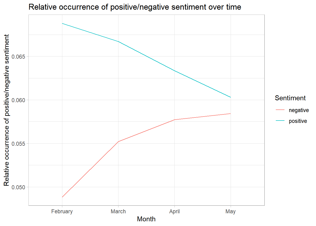
12.5.0.2 Organic dictionary
Given the oftentimes very limited validity of off-the-shelf dictionaries, we may often want to or have to develop our own dictionaries.
So-called organic dictionaries consist of specially created word lists appropriate for your research design and data see, for example, Muddiman et al. (2019).
For example, you may want to know how often newspapers use anxiety-related language to describe the issue of immigration.
Imagine that you have already developed your own dictionary and now want to look up the occurrence of these words to draw inferences about the construct you are interested in (anxiety-related language):9
dict_fear <- dictionary(list(fear = c("anxiety", "anxious", "afraid", "crisis",
                                        "terror", "threat", "carnage",
                                       "disaster", "horror", "tear",
                                       "cry", "nightmare", "kill", "death",
                                       "monster", "defeat", "crime", "violence",
                                       "violent")))
dict_fear
## Dictionary object with 1 key entry.
## - [fear]:
## - anxiety, anxious, afraid, crisis, terror, threat, carnage, disaster, horror, tear, cry, nightmare, kill, death, monster, defeat, crime, violence, violentWe apply the exact same logic to look up features of this organic dictionary in our texts:
sentiment_grouped_relative <- dfm_group(dfm, groups = month) %>%
  dfm_weight(scheme = "prop") %>%
  dfm_lookup(dictionary = dict_fear)
sentiment_grouped_relative
## Document-feature matrix of: 4 documents, 1 feature (0.00% sparse) and 1 docvar.
## features
## docs fear
## 2 0.001972266
## 3 0.002175917
## 4 0.002778979
## 5 0.002581006Transforming the results to long format, we can now visualize our findings:
plot <- convert(sentiment_grouped_relative, to = "data.frame")
plot <- melt(plot, id.vars = "doc_id")
ggplot(plot, aes(x = doc_id, y = value, group = variable, colour = variable)) +
  geom_line() +
  ylim(0, .01) +
  scale_x_discrete("Month", labels = c("February", "March", "April", "May"))+
  labs(y = "Relative occurrence of anxiety-related language",
       title = "Relative occurrence of anxiety-related language over time",
       colour = "Anxiety-related language") +
 theme_light()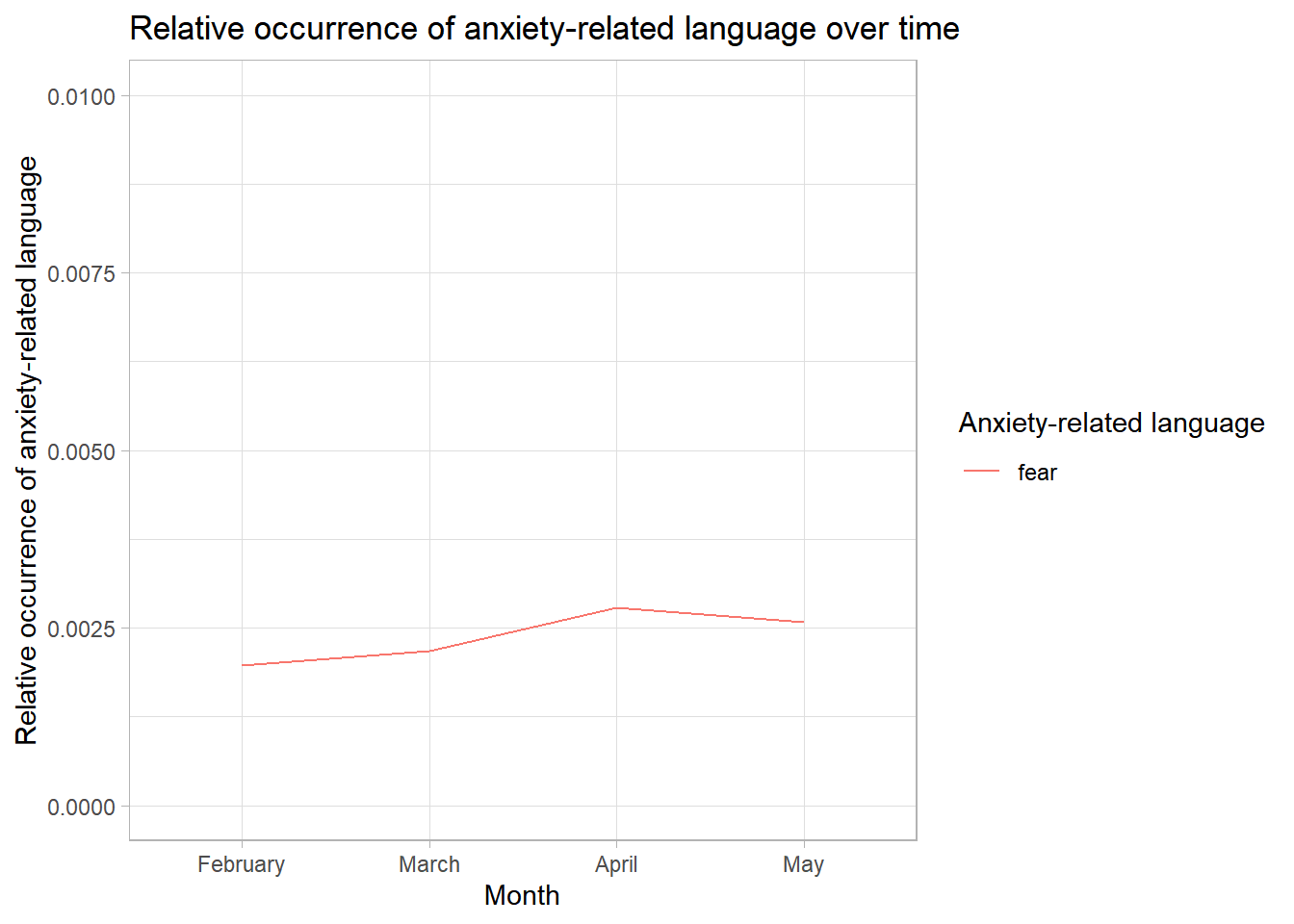
We find a very small increase in anxiety-related language. However, please note: Such features are almost never mentioned (see the small maximum value of the y axis).
12.6 Take Aways
Vocabulary:
- Keywords-in-Context or Keywords-in-Context-Analysis: Feature co-occurrences around a specific keyword.
- Co-Occurrences or Co-Occurrences-Analysis: Feature co-occurrences in a specific text.
- Dictionaries: Lists of words. Based on the manifest occurrence of these words, we draw conclusions about the occurrence of a latent construct, for example sentiment.
- Off-the-shelf dictionaries: Existing lists of words, often developed for other types of texts or topics.
- Organic dictionaries: Word lists you created specifically for your type of text, topic, or construct of interest.
Commands:
- Counting documents & features: ndoc(), nfeat()
- Analyzing feature occurrences: featfreq(), topfeatures(), textstat_frequency(), dfm_weight(), textplot_wordcloud(), dfm_group()
- Keywords-in-context: kwic()
- Co-occurrence analysis: fcm(), fcm_select(), textplot_network()
- Transforming quanteda objects to other types of objects: convert()
- Dictionary analysis: dictionary()
12.7 More tutorials on this
You still have questions? The following tutorials & papers can help you with that:
12.8 Test your knowledge
You’ve worked through all the material of Tutorial 12? Let’s see it - the following tasks will test your knowledge.
For this task, we’ll work with a new corpus: speeches_sotu.rda. The corpus includes “State of the Union Addresses” from US presidents since the 1790s.
You’ll find the corpus in OLAT (via: Materials / Data for R).
Source: The American Presidency Project, accessed via the quanteda corpus package.
load("corpus_sotu.rda")12.8.1 Task 12.1
Writing the corresponding R code, tokenize the corpus to sentences (not words) and save your result in a new object called data_new.
12.8.2 Task 12.2
Writing the corresponding R code, find out in how many sentences presidents use the term “United States”, i.e., in how many sentences the feature United States occurs.
This is where you’ll find Solutions for tutorial 12.
Let’s keep going: Tutorial 13: Topic Modeling
Note how we have more features than in the previous tutorial - we haven’t applied stemming, which is why features with a similar stem have not been transformed to the same stem↩︎
This is, of course, not a good example for such a dictionary. In fact, developing a good organic dictionary takes a lot of time and resources. Take the example as what it is: an example↩︎