5 Tutorial 5: Inspecting & transforming objects
After working through Tutorial 5, you’ll…
- understand how to inspect (elements of) objects
- understand how to edit (elements of) objects
For this tutorial, we’ll again use the data set “data_tutorial3.csv” (via OLAT/Materials/Data for R). The data set has already been introduced and explained in Tutorial 3: Objects & structures in R, so I won’t go into detail here.
survey <- read.csv2("data_tutorial3.csv", header = TRUE)By now, you should already know several ways of inspecting an object:
- Simply call the object’s name (or use print()):
survey## name age date outlet outlet_use outlet_trust
## 1 Alexandra 20 2021-09-09 TV 2 5
## 2 Alex 25 2021-09-08 Online 3 5
## 3 Maximilian 29 2021-09-09 Zeitung 4 1
## 4 Moritz 22 2021-09-06 TV 2 2
## 5 Vanessa 25 2021-09-07 Online 1 3
## 6 Andrea 26 2021-09-09 Online 3 4
## 7 Fabienne 26 2021-09-09 TV 3 2
## 8 Fabio 27 2021-09-09 Online 0 1
## 9 Magdalena 8 2021-09-08 Online 1 4
## 10 Tim 26 2021-09-07 TV NA 2
## 11 Alex 27 2021-09-09 Online NA 2
## 12 Tobias 26 2021-09-07 Online 2 2
## 13 Michael 25 2021-09-09 Online 3 2
## 14 Sabrina 27 2021-09-08 Online 1 2
## 15 Valentin 29 2021-09-09 TV 1 5
## 16 Tristan 26 2021-09-09 TV 2 5
## 17 Martin 21 2021-09-09 Online 1 2
## 18 Anna 23 2021-09-08 TV 3 3
## 19 Andreas 24 2021-09-09 TV 2 5
## 20 Florian 26 2021-09-09 Online 1 5- Use the View() command to inspect the object in a separate tab in the window “Script”:
View(survey)Image: Data set survey
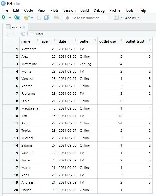
- Or use head(), which prints out the first elements of an object:
head(survey)## name age date outlet outlet_use outlet_trust
## 1 Alexandra 20 2021-09-09 TV 2 5
## 2 Alex 25 2021-09-08 Online 3 5
## 3 Maximilian 29 2021-09-09 Zeitung 4 1
## 4 Moritz 22 2021-09-06 TV 2 2
## 5 Vanessa 25 2021-09-07 Online 1 3
## 6 Andrea 26 2021-09-09 Online 3 45.1 Inspecting objects
5.1.1 Inspecting scalars
Inspecting scalars is easy, given that they only consist of a single value. Simply call the object. Here, we’ll use the object number consisting of the single value 3 as an example:
number <- 3
number
## [1] 35.1.2 Inspecting vectors
Let’s say you don’t have a single number but a row of numbers consisting of numeric data, e.g., the numbers from 1 to 20. This data is saved as the vector numbers:
numbers <- c(1:20)If you want to inspect all elements of numbers, again, simply call the object:
numbers## [1] 1 2 3 4 5 6 7 8 9 10 11 12 13 14 15 16 17 18 19 20However, maybe you only want to know the value of the first or second element of numbers - in this case, the first or second number.
In this case, we can use indexing to retrieve the corresponding element of numbers. In short, you tell R to only retrieve certain elements according to their position, i.e., their index. To do so, we use square brackets [].4
Let’s say we want to retrieve the first element of numbers:
numbers[1]## [1] 1… now it’s second:
numbers[2]## [1] 2.. and now the first, third, and fifth element:
numbers[c(1,3,5)]## [1] 1 3 5.. and, lastly, the first to seventh element as well as the element on position thirteen:
numbers[c(1:8,13)]## [1] 1 2 3 4 5 6 7 8 13As you see, you only need to remember some rules:
- Objects can be indexed by their position.
- You can either specify separate positions or, using the colon :, retrieve elements on several positions in a row.
5.1.3 Inspecting data frames
Remember that data frames consist of vectors of the same length.
Take, for instance, our data set survey: Its columns describe variables, its rows describe observations.
head(survey)## name age date outlet outlet_use outlet_trust
## 1 Alexandra 20 2021-09-09 TV 2 5
## 2 Alex 25 2021-09-08 Online 3 5
## 3 Maximilian 29 2021-09-09 Zeitung 4 1
## 4 Moritz 22 2021-09-06 TV 2 2
## 5 Vanessa 25 2021-09-07 Online 1 3
## 6 Andrea 26 2021-09-09 Online 3 4In difference to scalars and vectors, we can inspect elements from data frames both by indexing/their position and by their name.
5.1.3.1 Inspection by indexing/position
Say we want to get the name of the seventh respondent in our survey. We know that:
- the first column contains data on respondents’ names
- data for the respondent we are interested in (respondent number 7) is saved in the seventh row
Image: Data set survey
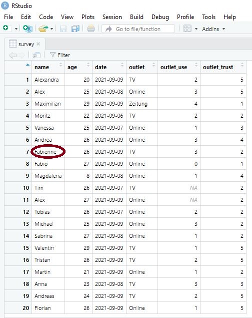
We can now access this value by its position using square brackets [], similar to vectors. Here,
- the first element in square brackets contains the row number(s)
- the second element in square brackets contains the column number(s)
Thus, if we want to retrieve data from the seventh row and the first column, we can do so via indexing:
survey[7,1]## [1] "Fabienne"In turn, if you do not want to retrieve a single value, but for instance all values for a specific respondent or all values for a specific variable, you could do the same via indexing.
For instance, this command retrieves all answers for the respondent called “Fabienne” (respondent number seven):
survey[7,]## name age date outlet outlet_use outlet_trust
## 7 Fabienne 26 2021-09-09 TV 3 2This command, in turn, retrieves all answers for the variable called “names” (column number one):
survey[,1]## [1] "Alexandra" "Alex" "Maximilian" "Moritz" "Vanessa" "Andrea" "Fabienne" "Fabio"
## [9] "Magdalena" "Tim" "Alex" "Tobias" "Michael" "Sabrina" "Valentin" "Tristan"
## [17] "Martin" "Anna" "Andreas" "Florian"5.1.3.2 Inspection by name
Another way of accessing elements is by their name. For instance, we could retrieve the variable “name” by simply using the variable name: We specify the object we want to access, the data frame survey, to then retrieve the column name via the operator $:
survey$name## [1] "Alexandra" "Alex" "Maximilian" "Moritz" "Vanessa" "Andrea" "Fabienne" "Fabio"
## [9] "Magdalena" "Tim" "Alex" "Tobias" "Michael" "Sabrina" "Valentin" "Tristan"
## [17] "Martin" "Anna" "Andreas" "Florian"5.1.3.3 Inspection by index/positioning and name
You will often retrieve data via a mix of indexing/positioning and data retrieval via column names.
For instance, if you have a data set with many different variables, you may not want to count the exact position of the variable of interest to you. In this case, it may be more useful to index rows by their position but columns by their name like so:
survey[7,c("name")]## [1] "Fabienne"Or you could simply retrieve the variable itself to then get the 7th element of the corresponding vector (knowing that observation number seven belongs to “Fabienne”):
survey$name[7]## [1] "Fabienne"In short: As with many problems in R, there isn’t just one solution - many variations of code will lead to the same solution (but may differ in efficiency).
5.1.4 Inspecting lists
Lastly, you can also inspect lists according to their position (or name).
Let’s create a list consisting of the following two elements:
- the data frame survey
- the vector numbers
list <- list(survey,numbers)You can now access each element of this list via its position. For instance, you could retrieve the second element of list, here the vector numbers, using double square brackets:
list[[2]]## [1] 1 2 3 4 5 6 7 8 9 10 11 12 13 14 15 16 17 18 19 20We could also give each element of your list list a name via name() to then access elements within list via their name:
names(list) <- c("survey", "numbers")
list["numbers"]
## $numbers
## [1] 1 2 3 4 5 6 7 8 9 10 11 12 13 14 15 16 17 18 19 205.2 Transforming objects
Now that we know that objects in R can by inspected/accessed by position and name, we also (almost) know how to transform data.
In many cases, we need to change existing objects in our working environment - for instance to filter data sets by conditions or to change specific values with an existing object.
5.2.1 Transforming scalars
In the case of scalars, we can simply overwrite our data. Since scalars consist of a single value, this is easily done:
word <- "hello"
word
## [1] "hello"word <- "goodbye"
word## [1] "goodbye"5.2.2 Tranforming vectors
We know that we can access vectors via indexing/their position.
Let’s first take the simple case that we want to change all elements belonging to a vector. For instance, we have a vector numbers that consists of all numbers between 1 to 20:
numbers <- c(1:20)
numbers
## [1] 1 2 3 4 5 6 7 8 9 10 11 12 13 14 15 16 17 18 19 20We can edit all values of numbers by, again, overwriting the vector:
numbers <- numbers + 1
numbers
## [1] 2 3 4 5 6 7 8 9 10 11 12 13 14 15 16 17 18 19 20 21However, if we only want to change a specific value within numbers, we need to do so via indexing. Say that we only want to change the second number in the vector:
numbers[2] <- 100
numbers
## [1] 2 100 4 5 6 7 8 9 10 11 12 13 14 15 16 17 18 19 20 21We can also, of course, change several elements within a vector. For instance, we may want to also replace the first and the last number:
numbers[c(1,20)] <- 0
numbers
## [1] 0 100 4 5 6 7 8 9 10 11 12 13 14 15 16 17 18 19 20 05.2.3 Transforming data frames
The same logic applies to changing values in data frames.
Using the survey data set, we may for example want to only include specific variables or only selected observations (filter data set by condition). Or we may want to change variables, for instance transform the variable on trust in news media scores to low and high trust instead of numeric values between 1 to 5 (change specific values).
5.2.3.1 Including/excluding columns of data frames
Say we want to use the data set survey, but only want to use the variables name and age.
For a better overview, we decide to create a new data set called survey_new, including only the variables name and age from the object data.
How would we do this?
5.2.3.1.1 Option 1: Indexing/selection via position
We only include selected variables via their position. We know that the variables name and age are saved in the first and second column of our object data, thus:
survey_new <- survey[,c(1:2)]
str(survey_new)
## 'data.frame': 20 obs. of 2 variables:
## $ name: chr "Alexandra" "Alex" "Maximilian" "Moritz" ...
## $ age : int 20 25 29 22 25 26 26 27 8 26 ...We could also specify those columns that we want to exclude. The negative operator - guarantees that all columns following it will be excluded:
survey_new <- survey[,-c(3:6)]
str(survey_new)
## 'data.frame': 20 obs. of 2 variables:
## $ name: chr "Alexandra" "Alex" "Maximilian" "Moritz" ...
## $ age : int 20 25 29 22 25 26 26 27 8 26 ...5.2.3.1.2 Option 2: Selection via name
Again, the more variables your data frame contains, the more prone to errors selection via a variable’s position. In many cases, it may just be easier to select variables we want to include via the variable’s name:
survey_new <- survey[,c("name", "age")]
str(survey_new)
## 'data.frame': 20 obs. of 2 variables:
## $ name: chr "Alexandra" "Alex" "Maximilian" "Moritz" ...
## $ age : int 20 25 29 22 25 26 26 27 8 26 ...5.2.3.2 Including/excluding rows of data frames
In addition, we may want to only keep or analyze selected rows (in this data set: observations).
Imagine that we want to include only those respondents that are older than 21 years.5 While we could also do this via indexing, i.e., write down all row numbers of respondents older than 21 years, this often becomes highly inefficient and prone to errors for many observations (imagine having to do such counting if your data set includes 1,000 observations).
Instead, we work with logical conditions to select rows. In principle, we ask R to consider a specific column - here, the variable survey$age - and only consider those rows where values for this variable take on values higher than 21.
I’ll show you two examples for this in the following.
5.2.3.2.1 Option 1
A first option is to simply specify necessary conditions for all columns and rows for the object survey.
In this case, we want R to include only rows where survey$age takes on values higher than 21. However, we also want R to consider all variables since we do not want to exclude specific variables for our dataset (we want to reduce the number of observations, not the variables which were considered.)
We therefore specify conditions for rows, but not for columns:
survey_new <- survey[survey$age>21,]
str(survey_new)
## 'data.frame': 17 obs. of 6 variables:
## $ name : chr "Alex" "Maximilian" "Moritz" "Vanessa" ...
## $ age : int 25 29 22 25 26 26 27 26 27 26 ...
## $ date : chr "2021-09-08" "2021-09-09" "2021-09-06" "2021-09-07" ...
## $ outlet : chr "Online " "Zeitung" "TV" "Online " ...
## $ outlet_use : int 3 4 2 1 3 3 0 NA NA 2 ...
## $ outlet_trust: int 5 1 2 3 4 2 1 2 2 2 ...We could, of course, also combine several conditions. For instance, if we only want to include students older than 21 who also mainly use TV according to the variable outlet_use to get information, we would write the following code:
survey_new <- survey[survey$age>21 & survey$outlet=="TV",]
str(survey_new)
## 'data.frame': 7 obs. of 6 variables:
## $ name : chr "Moritz" "Fabienne" "Tim" "Valentin" ...
## $ age : int 22 26 26 29 26 23 24
## $ date : chr "2021-09-06" "2021-09-09" "2021-09-07" "2021-09-09" ...
## $ outlet : chr "TV" "TV" "TV" "TV" ...
## $ outlet_use : int 2 3 NA 1 2 3 2
## $ outlet_trust: int 2 2 2 5 5 3 55.2.3.2.2 Option 2: dplyr
Another option is using the tidyverse, in particular the dplyr package.
The so-called tidyverse has become known as a collection of different R packages especially useful and accessible for R “beginners”6.
In the following, I’ll give you a short introduction into the tidyverse (especially dplyr for data wrangling and ggplot for data visualization in subsequent tutorials), but not an overall introduction. For more detailed sources on this, see
- The tidyverse Website, especially Wickham’s book R for data science
- Tutorial 12: Tidy data by G. Grolemund und H. Wickham
Dplyr is one of the most popular packages belonging to the tidyverse. It contains a lot of really helpful functions for data manipulation, out of which I will only mention a few. In particular, the pipe operator %>% has a central function.
Remember how we usually specify the arguments of a function: We call the function and specify the argument onto which we pass certain values.
For instance, here we pass the value survey$age to the argument x for the function mean():
mean(x = survey$age)## [1] 24.4We could also not even specify the name of the argument but simply include values for each argument in the right order, based on which R assumes that survey$age should be used as the value for x since it is the first value passed onto the function:
mean(survey$age)## [1] 24.4Moreover, if we want to use several functions, we have to nest them. For instance, the following code calculates the mean of age and then rounds the results to zero decimals:
round(mean(survey$age),0)## [1] 24The advantage of the pipe operator and the way dplyr works is that we do not have the nest functions - which is prone to errors as you may easily forget a bracket closing functions, for example. Instead, we simply specify the functions we want to use one after another.
The pipe operator %>% takes a certain object which is then passed over to one or several functions to its right. Results will be the same, but writing and nesting functions may be easier for you.
To use dplyr, you first have to install and activate the package. For help, see this useful cheat sheet on dplyr.
install.packages("dplyr")
library("dplyr")
Let’s take the same example as before: We want to include include those observations from the object survey where respondents said that they were older than 21 years.
To do this, we can use dplyr’s filter() function:
survey_new <- survey %>% filter(age > 21)
str(survey_new)
## 'data.frame': 17 obs. of 6 variables:
## $ name : chr "Alex" "Maximilian" "Moritz" "Vanessa" ...
## $ age : int 25 29 22 25 26 26 27 26 27 26 ...
## $ date : chr "2021-09-08" "2021-09-09" "2021-09-06" "2021-09-07" ...
## $ outlet : chr "Online " "Zeitung" "TV" "Online " ...
## $ outlet_use : int 3 4 2 1 3 3 0 NA NA 2 ...
## $ outlet_trust: int 5 1 2 3 4 2 1 2 2 2 ...How does dplyr work?
- We define the object with which we want to work: the data frame survey
- We pass on the object survey to our pipeline: %>%
- We filter the data set, i.e., keep only those observations where respondents are older than 21 years. We do not have to define the object - note that we only specify age instead of survey$age. We already told R to only use data from the object survey: filter(age > 21)
- We assign the result a new object survey_new: survey <-
One of the clearest advantages of dplyr is that we can efficiently nest functions: You can do different types of data manipulation within the same pipeline.
Say you want to first filter the data frame by age (i.e., only keep respondents older than 21) and then by favorite information outlet (i.e., only keep respondents getting their information from TV).
survey_new <-  survey %>%
  filter(age > 21) %>%
  filter(outlet == "TV")
str(survey_new)
## 'data.frame': 7 obs. of 6 variables:
## $ name : chr "Moritz" "Fabienne" "Tim" "Valentin" ...
## $ age : int 22 26 26 29 26 23 24
## $ date : chr "2021-09-06" "2021-09-09" "2021-09-07" "2021-09-09" ...
## $ outlet : chr "TV" "TV" "TV" "TV" ...
## $ outlet_use : int 2 3 NA 1 2 3 2
## $ outlet_trust: int 2 2 2 5 5 3 55.2.3.3 Including/excluding columns and rows of data frames
In some cases, you may also want to reduce your data frame to specific columns and rows.
Let’s assume you want to reduce the object survey to (a) respondents older than 21 years and (b) the variables name and age.
Again, different approaches for doing this exist, but the logic is the same:
survey_new <- survey[(survey$age>21), c("name", "age")]
str(survey_new)
## 'data.frame': 17 obs. of 2 variables:
## $ name: chr "Alex" "Maximilian" "Moritz" "Vanessa" ...
## $ age : int 25 29 22 25 26 26 27 26 27 26 ...Or, using the tidyverse approach using the functions filter() and select():
survey_new <-  survey %>%
  filter(age > 21) %>%
  select(name, age)
str(survey_new)
## 'data.frame': 17 obs. of 2 variables:
## $ name: chr "Alex" "Maximilian" "Moritz" "Vanessa" ...
## $ age : int 25 29 22 25 26 26 27 26 27 26 ...5.2.3.4 Transforming values in data frames
The same logic applied for transforming existing data.
Let’s say that we want to transform the variable outlet_trust in the object survey.
Remember: The variable indicates how much each student trusts a specific media outlet described in the variable outlet (from 1 = not at all to 5 = very much).
Instead of numeric values ranging from 1 to 5, we want to create a new variable named survey$outlet_trust_new which should include:
- “low trust” instead of the numeric values 1 and 2
- “medium trust” instead of the numeric value 3
- “high trust” instead of the numeric values 4 and 5
5.2.3.5 Option 1
- First, we create a new variable called outlet_trust_new which only consists of missing values.
- Next, only for those observations where outlet_trust takes on the values 1 and 2, we transform outlet_trust_new to take on the value “low trust”.
- Next, only for those observations where outlet_trust takes on the value 3, we transform outlet_trust_new to take on the value “medium trust”.
- Lastly, only for those observations where outlet_trust takes on the values 4 and 5, we transform outlet_trust_new to take on the value “high trust”.
In code, this looks as follows:
#create empty variable
survey$outlet_trust_new <- NA

#transform low trust scores
survey$outlet_trust_new[survey_new$outlet_trust==1|survey_new$outlet_trust==2] <- "low trust"

#transform medium trust scores
survey$outlet_trust_new[survey_new$outlet_trust==3] <- "medium trust"

#transform high trust scores
survey$outlet_trust_new[survey_new$outlet_trust==4|survey_new$outlet_trust==5] <- "high trust"

#inspect results
str(survey)
## 'data.frame': 20 obs. of 7 variables:
## $ name : chr "Alexandra" "Alex" "Maximilian" "Moritz" ...
## $ age : int 20 25 29 22 25 26 26 27 8 26 ...
## $ date : chr "2021-09-09" "2021-09-08" "2021-09-09" "2021-09-06" ...
## $ outlet : chr "TV" "Online " "Zeitung" "TV" ...
## $ outlet_use : int 2 3 4 2 1 3 3 0 1 NA ...
## $ outlet_trust : int 5 5 1 2 3 4 2 1 4 2 ...
## $ outlet_trust_new: chr NA NA NA NA ...5.2.3.6 Option 2
Using dplyr, we do the same thing - but use the %>% pipeline:
#create empty variable
survey$outlet_trust_new <- NA

#transform all trust scores in the same pipeline
survey <- survey %>%
  mutate(outlet_trust_new=replace(outlet_trust_new, outlet_trust<=2, "low trust")) %>%
  mutate(outlet_trust_new=replace(outlet_trust_new, outlet_trust==3, "medium trust")) %>%
  mutate(outlet_trust_new=replace(outlet_trust_new, outlet_trust>=4, "high trust"))

#inspect results
str(survey)
## 'data.frame': 20 obs. of 7 variables:
## $ name : chr "Alexandra" "Alex" "Maximilian" "Moritz" ...
## $ age : int 20 25 29 22 25 26 26 27 8 26 ...
## $ date : chr "2021-09-09" "2021-09-08" "2021-09-09" "2021-09-06" ...
## $ outlet : chr "TV" "Online " "Zeitung" "TV" ...
## $ outlet_use : int 2 3 4 2 1 3 3 0 1 NA ...
## $ outlet_trust : int 5 5 1 2 3 4 2 1 4 2 ...
## $ outlet_trust_new: chr "high trust" "high trust" "low trust" "low trust" ...5.3 Take Aways
- Inspecting objects:
- simply type in the object’s name, use print(), View(), str(), or head()
- to retrieve elements of a vector: vector[number of element]
- to retrieve elements of a data frame:
- for specific rows: data frame[number of row(s), ]
- for specific columns: data frame[ ,number of column(s) ] OR data frame$column
- for values in specific rows and columns: data frame[number of row(s), number of column(s)] OR data frame$column[number of rows(s)]
- for lists: list[[number of list element]] OR list$name of list element
- Transforming objects:
- Useful commands via dplyr, for instance: %>%, select(), filter(), mutate(), replace()
5.4 More tutorials on this
You still have questions? The following tutorials & papers can help you with that:
5.5 Test your knowledge
You’ve worked through all the material of Tutorial 5? Let’s see it - the following tasks will test your knowledge.
Since we are getting closer to October and thus Halloween season, we’ll work with a data set from fivethirthyeight on The Ultimate Halloween Candy Power Ranking.
In short, the data contains an online survey in which participants were asked to choose their favorite out of two different candy types. The data is accessible via a Creative Commons Attribution 4.0 International License here. You’ll have to copy the data into a “.txt” file. Else, you can also download the data from OLAT (via: Materials / Data for R, file called data_tutorial4.txt).
The data includes a range of variables, including
- the name of each candy bar: competitorname
- whether the candy bar contains chocolate: chocolate
- whether the candy bar contains fruit flavor: fruity
- whether the candy bar contains caramel: caramel
- the unit price percentile the candy bar is in compared to the rest of the set: pricepercent
5.5.1 Task 5.1
Read the data set into R. Writing the corresponding R code, find out
- how many observations and how many variables the data set contains.
5.5.2 Task 5.2
Writing the corresponding R code, find out
- how many candy bars contain chocolate.
- how many candy bars contain fruit flavor.
5.5.3 Task 5.3
Writing the corresponding R code, find out
- the name(s) of candy bars containing both chocolate and fruit flavor.
5.5.4 Task 5.4
Create a new data frame called data_new. Writing the corresponding R code,
- reduce the data set only observations containing chocolate but not caramel. The data set should also only include the variables competitorname and pricepercent.
- round the variable pricepercent to two decimals.
- sort the data by pricepercent in descending order, i.e., make sure that candy bars with the highest price are on top of the data frame and those with the lowest price on the bottom.
The corresponding data frame should look like this:
##                 competitorname pricepercent
## 1              Nestle Smarties         0.98
## 2            Hershey's Krackel         0.92
## 3     Hershey's Milk Chocolate         0.92
## 4       Hershey's Special Dark         0.92
## 5                  Mr Good Bar         0.92
## 6                       Mounds         0.86
## 7                     Whoppers         0.85
## 8                   Almond Joy         0.77
## 9          Nestle Butterfinger         0.77
## 10               Nestle Crunch         0.77
## 11         Peanut butter M&M's         0.65
## 12                       M&M's         0.65
## 13                 Peanut M&Ms         0.65
## 14   Reese's Peanut Butter cup         0.65
## 15              Reese's pieces         0.65
## 16 Reese's stuffed with pieces         0.65
## 17                3 Musketeers         0.51
## 18             Charleston Chew         0.51
## 19                Junior Mints         0.51
## 20                     Kit Kat         0.51
## 21        Tootsie Roll Juniors         0.51
## 22                 Tootsie Pop         0.32
## 23     Tootsie Roll Snack Bars         0.32
## 24          Reese's Miniatures         0.28
## 25            Hershey's Kisses         0.09
## 26                     Sixlets         0.08
## 27        Tootsie Roll Midgies         0.01
This is where you’ll find solutions for tutorial 5.
Let’s keep going: Tutorial 6: Control structures & functions in R.
We could have also done that for the scalar word. However, since the object only contains one value, this would not make much sense. To understand that, compare the commands word[1] and word[2]↩︎
Remember Tutorial 3.1.6? We’ve already encountered this kind of code!↩︎
Though I never met anyone who “finished” R, so remember that we are all beginners in R - or that we are all learning R, but are at different stages of doing so.↩︎