13 Tutorial 13: Topic Modeling

After working through Tutorial 13, you’ll…

understand how to use unsupervised machine learning in the form of topic modeling with R.

13.1 Preparing the corpus

Let’s use the same data as in the previous tutorials. You can find the corresponding R file in OLAT (via: Materials / Data for R) with the name immigration_news.rda.

Source of the data set: Nulty, P. & Poletti, M. (2014). “The Immigration Issue in the UK in the 2014 EU Elections: Text Mining the Public Debate.” Presentation at LSE Text Mining Conference 2014. Accessed via the quanteda corpus package.

load("immigration_news.rda")

Again, we use some preprocessing steps to prepare the corpus for analysis.

Please remember that the exact choice of preprocessing steps (and their order) depends on your specific corpus and question - it may thus differ from the approach here.

We save the publication month of each text (we’ll later use this vector as a document level variable)
We remove the pattern for a line break \n.
We tokenize our texts, remove punctuation/numbers/URLs, transform the corpus to lowercase, and remove stopwords.
We apply relative pruning
We save the result as a document-feature-matrix called dfm.

library("stringr")
library("quanteda")

#extracting the publication month
data$month <- str_extract(string = data$text, 
                          pattern = "[0-9]+ (january|february|march|april|may|june|july|august|september|october|november|december) 2014")
data$month <- str_extract(string = data$month, 
                          pattern = "january|february|march|april|may|june|july| august|september|october|november|december")

#turning the publication month into a numeric format
data$month[data$month=="february"] <- "2"
data$month[data$month=="march"] <- "3"
data$month[data$month=="april"] <- "4"
data$month[data$month=="may"] <- "5"

#removing the pattern indicating a line break
data$text <- gsub(pattern = "\n", replacement = " ", x = data$text)

#tokenization & removing punctuation/numbers/URLs etc.
tokens <- data$text %>%
          tokens(what = "word",
                 remove_punct = TRUE,
                 remove_numbers = TRUE,
                 remove_url = TRUE) %>%
          tokens_tolower() %>%
          tokens_remove(stopwords("english"))

#applying relative pruning
dfm <- dfm_trim(dfm(tokens), min_docfreq = 0.005, max_docfreq = 0.99, 
                docfreq_type = "prop", verbose = TRUE)

## Removing features occurring:

##   - in fewer than 14.165 documents: 33,992

##   - in more than 2804.67 documents: 2

##   Total features removed: 33,994 (86.8%).

#This is our dfm
dfm

## Document-feature matrix of: 2,833 documents, 5,162 features (97.14% sparse) and 0 docvars.
##        features
## docs    support ukip continues grow labour heartlands miliband scared leo mckinstry
##   text1       2    7         1    1      8          2        4      1   1         1
##   text2       0    1         0    0      0          0        0      0   0         0
##   text3       0    1         0    0      0          0        0      0   0         0
##   text4       0    0         0    0      0          0        0      0   0         0
##   text5       0    1         0    0      0          0        0      0   0         0
##   text6       0    0         0    0      0          0        0      0   0         0
## [ reached max_ndoc ... 2,827 more documents, reached max_nfeat ... 5,152 more features ]

Let’s make sure that we did remove all feature with little informative value.

To check this, we quickly have a look at the top features in our corpus (after preprocessing):

topfeatures(dfm, n = 20, scheme = "docfreq")

##           ©      rights    reserved        said         ltd immigration        news         one      people         may 
##        2085        2014        1970        1766        1704        1687        1545        1522        1520        1458 
##        last  newspapers        also          uk     britain       group          mr         new         can         now 
##        1262        1250        1190        1177        1142        1088        1086        1085        1082        1076

It seems that we may have missed some things during preprocessing. For instance, the most frequent feature “©” or, similarly, “ltd”, “rights”, and “reserved” probably signify some copy-right text that we could remove (since it may be a formal aspect of the data source rather than part of the actual newspaper coverage we are interested in).

We could remove them in an additional preprocessing step, if necessary:

dfm <- dfm_remove(dfm, c("©", "ltd", "rights", "reserved"))

13.2 Topic modeling: The basics

Topic modeling describes an unsupervised machine learning technique that exploratively identifies latent topics based on frequently co-occurring words. Thus, we attempt to infer latent topics in texts based on measuring manifest co-occurrences of words.

Unlike unsupervised machine learning, topics are not known a priori. Thus, we do not aim to sort documents into pre-defined categories (i.e., topics). Instead, we use topic modeling to identify and interpret previously unknown topics in texts.

Broadly speaking, topic modeling adheres to the following logic:

You as a researcher specify the presumed number of topics K thatyou expect to find in a corpus (e.g., K = 5, i.e., 5 topics). When running the model, the model then tries to inductively identify 5 topics in the corpus based on the distribution of frequently co-occurring features. An algorithm is used for this purpose, which is why topic modeling is a type of “machine learning”.

Important: The choice of K, i.e. whether I instruct my model to identify 5 or 100 topics, has a substantial impact on results. The smaller K, the more fine-grained and usually the more exclusive topics; the larger K, the more clearly topics identify individual events or issues. However, with a larger K topics are oftentimes less exclusive, meaning that they somehow overlap. You see: Choosing the number of topics K is one of the most important, but also difficult steps when using topic modeling.

The model generates two central results important for identifying and interpreting these 5 topics:

Word-topic matrix: This matrix describes the conditional probability of a feature being prevalent in a given topic. We often use it to inspect the top features of a topic (i.e., the features having the highest conditional probability for said topic) to label and interpret topics. In short, the matrix helps used to generate word lists that describe each topic.
Document Topic Matrix: This matrix describes the conditional probability of a topic being prevalent in a given document. We often use it to inspect the top documents of a topic (i.e., the documents having the highest conditional probability for said topic) to assign one or more main topics to articles. In short, the matrix helps used to generate topic lists that describe a document.

Importantly, all features are assigned a conditional probability > 0 and < 1 with which a feature is prevalent in a document, i.e., no cell of the word-topic matrix amounts to zero (although probabilities may lie close to zero). Similarly, all documents are assigned a conditional probability > 0 and < 1 with which a particular topic is prevalent, i.e., no cell of the document-topic matrix amounts to zero (although probabilities may lie close to zero).

In conclusion, topic models do not identify a single main topic per document. Instead, topic models identify the probabilities with which each topic is prevalent in each document. This is why topic models are also called mixed-membership models: They allow documents to be assigned to multiple topics and features to be assigned to multiple topics with varying degrees of probability. You as a researcher have to draw on these conditional probabilities to decide whether and when a topic or several topics are present in a document - something that, to some extent, needs some manual decision-making.

In this context, topic models often contain so-called background topics. These are topics that seem incoherent and cannot be meaningfully interpreted or labeled because, for example, they do not describe a single event or issue. Often, topic models identify topics that we would classify as background topics because of a similar writing style or formal features that frequently occur together. Such topics should be identified and excluded for further analysis. Thus, an important step in interpreting results of your topic model is also to decide which topics can be meaningfully interpreted and which are classified as background topics and will therefore be ignored. The more background topics a model generates, the less helpful it probably is for accurately understanding the corpus. Accordingly, a model that contains only background topics would not help identify coherent topics in our corpus and understand it. However, researchers often have to make relatively subjective decisions about which topics to include and which to classify as background topics.

In sum, please always be aware: Topic models require a lot of human (partly subjective) interpretation when it comes to…

the choice of K topics
the identification and exclusion of background topics
the interpretation and labeling of topics identified as relevant
the “assignment” of topics to documents

Since session 10 already included a short introduction to the theoretical background of topic modeling as well as promises/pitfalls of the approach, I will only summarize the most important take-aways here:

Things to consider when running your topic model.

There are no clear criteria for how you determine the number of topics K that should be generated. I would recommend you rely on statistical criteria (such as: statistical fit) and interpretability/coherence of topics generated across models with different K (such as: interpretability and coherence of topics based on top words).
Always (!) look at topics manually, for instance by drawing on top features and top documents. In the best possible case, topics’ labels and interpretation should be systematically validated manually (see following tutorial).
Think carefully about which theoretical concepts you can measure with topics. Be careful not to “over-interpret” results (see here for a critical discussion on whether topic modeling can be used to measure e.g. frames).¹⁰

As a recommendation (you’ll also find most of this information on the syllabus): The following texts are really helpful for further understanding the method:

Texts:

From a communication research perspective, one of the best introductions to topic modeling is offered by Maier et al. (2018)

Maier, D., Waldherr, A., Miltner, P., Wiedemann, G., Niekler, A., Keinert, A., Pfetsch, B., Heyer, G., Reber, U., Häussler, T., Schmid-Petri, H., & Adam, S. (2018). Applying LDA Topic Modeling in Communication Research: Toward a Valid and Reliable Methodology. Communication Methods and Measures, 12(2–3), 93–118. Link

Other than that, the following texts may be helpful:

Blei, D. M. (2012). Probabilistic topic models. Communications of the ACM, 55(4), 77–84. Link
Jacobi, C., van Atteveldt, W., & Welbers, K. (2016). Quantitative analysis of large amounts of journalistic texts using topic modelling. Digital Journalism, 4(1), 89–106. Link
Mohr, J. W., & Bogdanov, P. (2013). Introduction—Topic models: What they are and why they matter. Poetics, 41(6), 545–569. Link
Roberts, M. E., Stewart, B. M., Tingley, D., Lucas, C., Leder-Luis, J., Gadarian, S. K., Albertson, B., & Rand, D. G. (2014). Structural Topic Models for Open-Ended Survey Responses: STRUCTURAL TOPIC MODELS FOR SURVEY RESPONSES. American Journal of Political Science, 58(4), 1064–1082. Link
Schmidt, B. M. (2012) Words Alone: Dismantling Topic Modeling in the Humanities. Journal of Digital Humanities, 2(1). Link
Quinn, K. M., Monroe, B. L., Colaresi, M., Crespin, M. H., & Radev, D. R. (2010). How to Analyze Political Attention with Minimal Assumptions and Costs. American Journal of Political Science, 54(1), 209–228. Link
Wilkerson, J., & Casas, A. (2017). Large-Scale Computerized Text Analysis in Political Science: Opportunities and Challenges. Annual Review of Political Science, 20(1), 529–544. Link

13.3 How do I run a topic model in R?

In the following, we’ll work with the stm package Link and Structural Topic Modeling (STM). While a variety of other approaches or topic models exist, e.g., Keyword-Assisted Topic Modeling, Seeded LDA, or Latent Dirichlet Allocation (LDA) as well as Correlated Topics Models (CTM), I chose to show you Structural Topic Modeling.

STM has several advantages. Among other things, the method allows for correlations between topics. STM also allows you to explicitly model which variables influence the prevalence of topics. For example, you can calculate the extent to which topics are more or less prevalent over time, or the extent to which certain media outlets report more on a topic than others. Compared to at least some of the earlier topic modeling approaches, its non-random initialization is also more robust.

How do we calculate a topic model?

First, you need to get your DFM into the right format to use the stm package:

dfm_stm <- convert(dfm, to = "stm")

As an example, we will now try to calculate a model with K = 15 topics (how to decide on the number of topics K is part of the next sub-chapter). I want you to understand how topic models work more generally before comparing different models, which is why we more or less arbitrarily choose a model with K = 15 topics.

To run the topic model, we use the stm() command,which relies on the following arguments:

document: The argument tells the function to run the topic model using articles from our dfm.
vocab: The argument tells the function to use the features saved in the dfm.
K: The argument tells the function to identify 15 topics.
verbose: The argument tells the function to tell us about the status quo of the process, i.e., which calculations are currently being performed.

library("stm")
model <- stm(documents = dfm_stm$documents,
         vocab = dfm_stm$vocab, 
         K = 15,
         verbose = TRUE)

Running the model will take some time (depending on, for instance, the computing power of your machine or the size of your corpus)

Let’s inspect the result:

plot(model)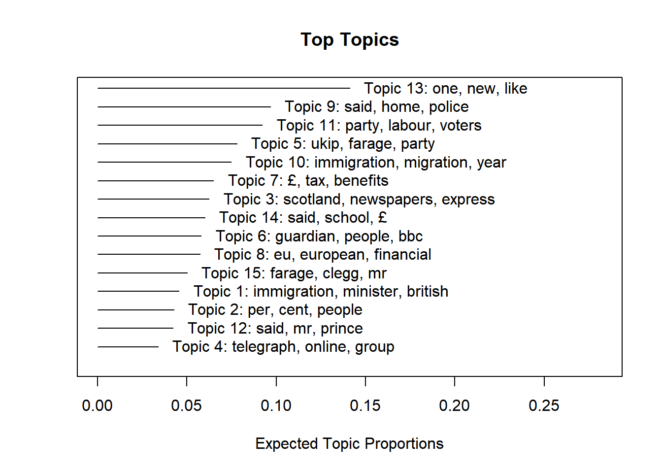

The plot() command visualizes the top features of each topic as well as each topic’s prevalence based on the document-topic-matrix:

The features displayed after each topic (Topic 1, Topic 2, etc.) are the features with the highest conditional probability for each topic. For example, we see that Topic 7 seems to concern taxes or finance: here, features such as the pound sign “£”, but also features such as “tax” and “benefits” occur frequently.
The x-axis (the horizontal line) visualizes what is called “expected topic proportions”, i.e., the conditional probability with with each topic is prevalent across the corpus. We can for example see that the conditional probability of topic 13 amounts to around 13%. This makes Topic 13 the most prevalent topic across the corpus. Topic 4 - at the bottom of the graph - on the other hand, has a conditional probability of 3-4% and is thus comparatively less prevalent across documents.

Let’s inspect the word-topic matrix in detail to interpret and label topics.

To do so, we can use the labelTopics command to make R return each topic’s top five terms (here, we do so for the first five topics):

labelTopics(model,topics = c(1:5), n=5)

## Topic 1 Top Words:
##       Highest Prob: immigration, minister, british, mr, said 
##       FREX: nanny, cable, cheap, brokenshire, metropolitan 
##       Lift: brokenshires, gita, tradesmen, lima, stewart 
##       Score: nanny, brokenshire, stewart, lima, cable 
## Topic 2 Top Words:
##       Highest Prob: per, cent, people, ethnic, britain 
##       FREX: ethnic, minority, cent, per, communities 
##       Lift: qualified, researchers, minorities, census, ethnic 
##       Score: cent, per, ethnic, qualified, minority 
## Topic 3 Top Words:
##       Highest Prob: scotland, newspapers, express, news, document 
##       FREX: scotland, scottish, sun, express, theexp 
##       Lift: 6en, ec3r, photo, salmonds, snp 
##       Score: photo, scotland, express, scottish, theexp 
## Topic 4 Top Words:
##       Highest Prob: telegraph, online, group, media, daily 
##       FREX: telegraph, teluk, dt, media, lords 
##       Lift: nelson, bulletin, dt, telegraph, teluk 
##       Score: telegraph, teluk, nelson, dt, media 
## Topic 5 Top Words:
##       Highest Prob: ukip, farage, party, said, mr 
##       FREX: racist, poster, posters, candidates, bnp 
##       Lift: thandi, henwood, lampitt, lizzy, mercer 
##       Score: farage, ukip, thandi, racist, lampitt

As you can see, R returns the top terms for each topic in four different ways. I would recommend concentrating on FREX weighted top terms. Roughly speaking, top terms according to FREX weighting show you which words are comparatively common for a topic and exclusive for that topic compared to other topics. Thus, top terms according to FREX weighting are usually easier to interpret.

For example, you can see that topic 2 seems to be about “minorities”, while the other topics cannot be clearly interpreted based on the most frequent 5 features.

If we now want to inspect the conditional probability of features for all topics according to FREX weighting, we can use the following code.

It creates a vector called topwords consisting of the 20 features with the highest conditional probability for each topic (based on FREX weighting). We primarily use these lists of features that “make up” a topic to label and interpret each topic. In principle, it contains the same information as the result generated by the labelTopics() command.

#Save top 20 features across topics and forms of weighting
labels <- labelTopics(model, n=20)
#only keep FREX weighting
topwords <- data.frame("features" = t(labels$frex))
#assign topic number as column name
colnames(topwords) <- paste("Topics", c(1:15))
#Return the result
topwords[1:5]

##        Topics 1    Topics 2     Topics 3  Topics 4   Topics 5
## 1         nanny      ethnic     scotland telegraph     racist
## 2         cable    minority     scottish     teluk     poster
## 3         cheap        cent          sun        dt    posters
## 4   brokenshire         per      express     media candidates
## 5  metropolitan communities       theexp     lords        bnp
## 6         elite  minorities       thesun    online       ukip
## 7         vince      groups      salmond      bill      ukips
## 8       wealthy  university    edinburgh  <U+7AB6>  candidate
## 9          lima       white    editorial     group     newark
## 10     employed    suggests        scots     daily    lampitt
## 11      workers       study      opinion      lord     racism
## 12      nannies      likely         alex   reading        mep
## 13      downing    research          snp      stel     ukip's
## 14       speech  proportion          yes   georgia      henry
## 15      citizen      survey independence     peers     farage
## 16    employers       asian            c  cardinal      sykes
## 17      theresa      census        javid questions   comments
## 18        james       black       border       tim  interview
## 19       employ       among      glasgow  <U+51B1>    farages
## 20      cleaner  population       thesuk     peter     thandi

However, as mentioned before, we should also consider the document-topic-matrix to understand our model. This matrix describes the conditional probability with which a topic is prevalent in a given document. We can use this information (a) to retrieve and read documents where a certain topic is highly prevalent to understand the topic and (b) to assign one or several topics to documents to understand the prevalence of topics in our corpus.

Here, we use make.dt() to get the document-topic-matrix(). As an example, we’ll retrieve the document-topic probabilities for the first document and all 15 topics.

theta <- make.dt(model)
theta[1,1:16]

##    docnum      Topic1     Topic2      Topic3      Topic4      Topic5      Topic6      Topic7     Topic8       Topic9
## 1:      1 0.003935035 0.04556144 0.004846942 0.003014408 0.009297329 0.004452513 0.005698955 0.00926361 3.567387e-05
##       Topic10   Topic11     Topic12     Topic13      Topic14   Topic15
## 1: 0.00426147 0.7872743 0.001564772 0.001601545 0.0009265871 0.1182654

Based on the results, we may think that topic 11 is most prevalent in the first document. In turn, by reading the first document, we could better understand what topic 11 entails.

13.4 How do I decide on the number of topics K that should be identified?

Now that you know how to run topic models: Let’s now go back one step.

Before running the topic model, we need to decide how many topics K should be generated. As mentioned during session 10, you can consider two criteria to decide on the number of topics K that should be generated:

Statistical fit
Interpretability of topics

It is important to note that statistical fit and interpretability of topics do not always go hand in hand. By relying on these criteria, you may actually come to different solutions as to how many topics seem a “good” choice. For example, studies show that models with good statistical fit are often difficult to interpret for humans and do not necessarily contain meaningful topics. Accordingly, it is up to you to decide how much you want to consider the statistical fit of models.

Moreover, there isn’t one “correct” solution for choosing the number of topics K. In some cases, you may want to generate “broader” topics - in other cases, the corpus may be better represented by generating more fine-grained topics using a larger K. That is precisely why you should always be transparent about why and how you decided on the number of topics K when presenting a study on topic modeling.

As an example, we will here compare a model with K = 4 and a model with K = 6 topics. This is merely an example - in your research, you would mostly compare more models (and presumably models with a higher number of topics K).

13.4.1 Criterion 1: Statistical fit

We can rely on the stm package to roughly limit (but not determine) the number of topics that may generate coherent, consistent results.

Using searchK() , we can calculate the statistical fit of models with different K.

The code used here is an adaptation of Julia Silge’s STM tutorial, available here. For simplicity, we only rely on two criteria here: the semantic coherence and exclusivity of topics, both of which should be as high as possible.

Semantic Coherence: tells you how coherent topics are, i.e., how often features describing a topic co-occur and topics thus appear to be internally coherent.
Exclusivity: tells you how exclusive topics are, i.e., how much they differ from each other and topics thus appear to describe different things.

We first calculate both values for topic models with 4 and 6 topics:

K <- c(4,6)
fit <- searchK(dfm_stm$documents, dfm_stm$vocab, K = K, verbose = TRUE)

We then visualize how these indices for the statistical fit of models with different K differ:

# Create graph
plot <- data.frame("K" = K, 
                   "Coherence" = unlist(fit$results$semcoh),
                   "Exclusivity" = unlist(fit$results$exclus))

# Reshape to long format
library("reshape2")
plot <- melt(plot, id=c("K"))
plot

##   K    variable      value
## 1 4   Coherence -45.537079
## 2 6   Coherence -52.288480
## 3 4 Exclusivity   8.626872
## 4 6 Exclusivity   8.894482

#Plot result
library("ggplot2")
ggplot(plot, aes(K, value, color = variable)) +
  geom_line(size = 1.5, show.legend = FALSE) +
  facet_wrap(~variable,scales = "free_y") +
  labs(x = "Number of topics K",
       title = "Statistical fit of models with different K")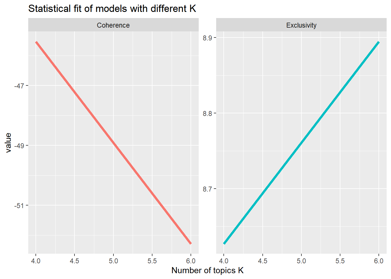

What does this graph tell us?

In terms of semantic coherence: The coherence of the topics decreases the more topics we have (the model with K = 6 does “worse” than the model with K = 4). In turn, the exclusivity of topics increases the more topics we have (the model with K = 4 does “worse” than the model with K = 6).

In sum, based on these statistical criteria only, we could not decide whether a model with 4 or 6 topics is “better”.

13.4.2 Criterion 2: Interpretability and relevance of topics

A second - and often more important criterion - is the interpretability and relevance of topics. Specifically, you should look at how many of the identified topics can be meaningfully interpreted and which, in turn, may represent incoherent or unimportant background topics. The more background topics a model has, the more likely it is to be inappropriate to represent your corpus in a meaningful way.

Here, we’ll look at the interpretability of topics by relying on top features and top documents as well as the relevance of topics by relying on the Rank-1 metric.

First, we compute both models with K = 4 and K = 6 topics separately.

model_4K <- stm(documents = dfm_stm$documents,
         vocab = dfm_stm$vocab, 
         K = 4,
         verbose = TRUE)
model_6K <- stm(documents = dfm_stm$documents,
         vocab = dfm_stm$vocab, 
         K = 6,
         verbose = TRUE)

1: Top Features

You have already learned that we often rely on the top features for each topic to decide whether they are meaningful/coherent and how to label/interpret them. We can also use this information to see how topics change with more or less K:

Let’s take a look at the top features based on FREX weighting:

#for K = 4
topics_4 <- labelTopics(model_4K, n=10)
topics_4 <- data.frame("features" = t(topics_4$frex))
colnames(topics_4) <- paste("Topics", c(1:4))
topics_4

##       Topics 1     Topics 2 Topics 3 Topics 4
## 1       police    migration     book   farage
## 2        nanny          net   prince     ukip
## 3       asylum      numbers    story   voters
## 4        court restrictions     film    party
## 5  deportation     increase    music    clegg
## 6     deported       merkel  theatre    nigel
## 7      illegal       growth features miliband
## 8        judge     migrants  america      lib
## 9     passport    countries american     vote
## 10    arrested      benefit  parents  farages

#for K = 6
topics_6 <- labelTopics(model_6K, n=10)
topics_6 <- data.frame("features" = t(topics_6$frex))
colnames(topics_6) <- paste("Topics", c(1:6))
topics_6

##        Topics 1     Topics 2 Topics 3      Topics 4  Topics 5 Topics 6
## 1      scotland          net     film         court    farage   indeed
## 2         nanny    migration      son        police      ukip  society
## 3      scottish      numbers  theatre         judge     party thatcher
## 4   brokenshire restrictions    music investigation     nigel      bbc
## 5         cable      figures  america     criminals elections   prince
## 6         cheap     increase facebook      criminal   farages margaret
## 7            ms       merkel    novel      arrested    voters    might
## 8       wealthy   bulgarians     love      officers      poll  ukraine
## 9  metropolitan    financial   father    passengers      dems   global
## 10          mrs           ft      art         serco  miliband   hitler

As you see, both models contain similar topics (at least to some extent):

Topic 2 in the model with K = 4 and Topic 2 in the model with K = 6 seem to be about migration numbers and their development over time.
Theme 3 in the model with K = 4 and Theme 3 in the model with K = 6 seem to be about culture and art; its unclear whether this topic actually deals with immigration.
Topic 4 in the model with K = 4 and Topic 5 in the model with K = 6 seem to be about the (former) UK politician Nigel Farage and the right-leaning party UKIP.

You could therefore consider the “new topic” in the model with K = 6 (here topic 1, 4, and 6): Are they relevant and meaningful enough for you to prefer the model with K = 6 over the model with K = 4?

2: Top documents

In addition, you should always read document considered representative examples for each topic - i.e., documents in which a given topic is prevalent with a comparatively high probability.

The findThoughts() command can be used to return these articles by relying on the document-topic-matrix. Here, we for example make R return a single document representative for the first topic (that we assumed to deal with deportation):

findThoughts(model_4K, data$text, topics=1, n=1)

## 
##  Topic 1: 
##          yashika bageerathis final appeal against deportation rejected by judge mark tran    theguardiancom 596 words 3 april 2014 guardiancouk grultd english c 2014 guardian news & media limited all rights reserved    lord justice richards refuses to grant emergency injunction as mauritian student 19 is taken to airport a judge has rejected a final appeal against the deportation of a 19-year-old mauritian student hours before she was due to depart heathrow lawyers for yashika bageerathi lodged papers with a judge at the high court seeking an emergency injunction to block her removal and give her time to take her case to the court of appeal as she was being driven to heathrow on wednesday to await her flight at 9pm lord justice richards refused to order a stay of deportation in a telephone hearing a spokesman for the oasis academy hadley in north london where bageerathi has been studying said she was set to fly out of terminal 4 on an air mauritius flight this will be the third attempt to send her back to mauritius in little over a week bageerathi was very distressed and worried the spokesman added he said she is on her way in the van but i really hope we can keep her here were encouraging everyone to tweet air mauritius and to phone them to stop this she was supposed to have gone on sunday but her supporters said air mauritius had refused to fly her out following an earlier refusal by british airways but despite a vocal campaign for bageerathi to stay so she can finish her a-levels the home office is adamant that she should return to mauritius on monday james brokenshire the immigration minister told the house of commons that the home office would not intervene he said her case had been through the proper legal process and the home offices decision that she did not need protection from violence or persecution in her homeland had been upheld brokenshire said that given the extent and level of judicial and other scrutiny the home secretary theresa may had decided not to intervene bageerathi has been held at yarls wood immigration removal centre near bedford since 19 march she came to the uk with her mother sister and brother in 2011 to escape a relative who was physically abusive and they claimed asylum last summer but the family were told they all faced the threat of deportation bageerathi is being deported without her mother and two siblings because as an adult her case was considered separate to theirs a petition calling on authorities to stop the deportation has gathered more than 175000 signatures on the website changeorg campaigners who include her schoolmates and the school principal said yashika bageerathi arrived in the uk along with her mother and brother in 2012 to escape abuse and danger in that time yashika has proved herself a model student and valuable member of the co

3: Rank-1 metric

A third criterion for assessing the number of topics K that should be calculated is the Rank-1 metric. The Rank-1 metric describes in how many documents a topic is the most important topic (i.e., has a higher conditional probability of being prevalent than any other topic).

By relying on the Rank-1 metric, we assign each document exactly one main topic, namely the topic that is most prevalent in this document according to the document-topic-matrix.

First, we retrieve the document-topic-matrix for both models.

theta_4K <- make.dt(model_4K)
theta_6K <- make.dt(model_6K)

We can now use this matrix to assign exactly one topic, namely that which has the highest probability for a document, to each document.

You should keep in mind that topic models are so-called mixed-membership models, i.e. every topic has a certain probability of appearing in every document (even if this probability is very low). By assigning only one topic to each document, we therefore lose quite a bit of information about the relevance that other topics (might) have for that document - and, to some extent, ignore the assumption that each document consists of all topics.

Nevertheless, the Rank1 metric, i.e., the absolute number of documents in which a topic is the most prevalent, still provides helpful clues about how frequent topics are and, in some cases, how the occurrence of topics changes across models with different K.

Let’s retrieve the metric:

#First, we generate an empty data frame for both models
data$Rank1_K4 <- NA #K = 4
data$Rank1_K6 <- NA #K = 6

#calculate Rank-1 for K = 4
for (i in 1:nrow(data)){
  column <- theta_4K[i,-1]
  maintopic <- colnames(column)[which(column==max(column))]
  data$Rank1_K4[i] <- maintopic
}
table(data$Rank1_K4)

## 
## Topic1 Topic2 Topic3 Topic4 
##    461    730    800    842

#calculate Rank-1 for K = 6
for (i in 1:nrow(data)){
  column <- theta_6K[i,-1]
  maintopic <- colnames(column)[which(column==max(column))]
  data$Rank1_K6[i] <- maintopic
}
table(data$Rank1_K6)

## 
## Topic1 Topic2 Topic3 Topic4 Topic5 Topic6 
##    203    505    530    417    780    398

What does this result tell us?

It tells us that all topics are comparably frequent across models with K = 4 topics and K = 6 topics, i.e., quite a lot of documents are assigned to individual topics.

Had we found a topic with very few documents assigned to it (i.e., a less prevalent topic), this might indicate that it is a background topic that we may exclude for further analysis (though that may not always be the case).

13.5 How do I include independent variables in my topic model?

Once we have decided on a model with K topics, we can perform the analysis and interpret the results. For simplicity, we now take the model with K = 6 topics as an example, although neither the statistical fit nor the interpretability of its topics give us any clear indication as to which model is a “better” fit.

As mentioned before, Structural Topic Modeling allows us to calculate the influence of independent variables on the prevalence of topics (and even the content of topics, although we won’t learn that here).

Suppose we are interested in whether certain topics occur more or less over time.

Thus, we want to use the publication month as an independent variable to see whether the month in which an article was published had any effect on the prevalence of topics.

To do exactly that, we need to add to arguments to the stm() command:

prevalence: the argument tells the function to model the prevalence of topics based on the month of publication. Here, we are simply going for a linear relationship between the prevalence of topics (dependent variable) and the month of publication (independent variable).
data: the argument tells the function where to find the independent variable’s values. In our case, this is the original data frame data, in which we had stored the texts and associated meta-information.

data$month <- as.numeric(data$month)
model <- stm(documents = dfm_stm$documents,
             vocab = dfm_stm$vocab, 
             K = 6,
             prevalence = ~month,
             data = data,
             verbose = TRUE)

Next, we can use estimateEffect() to plot the effect of the variable data$Month on the prevalence of topics.

effect <- estimateEffect(formula=~month, stmobj=model, metadata=data)

The results of this regression are most easily accessible via visual inspection. Here, we only consider the increase or decrease of the first three topics as a function of time for simplicity:

plot(effect, "month", method = "continuous", topics = c(1:3), model = model)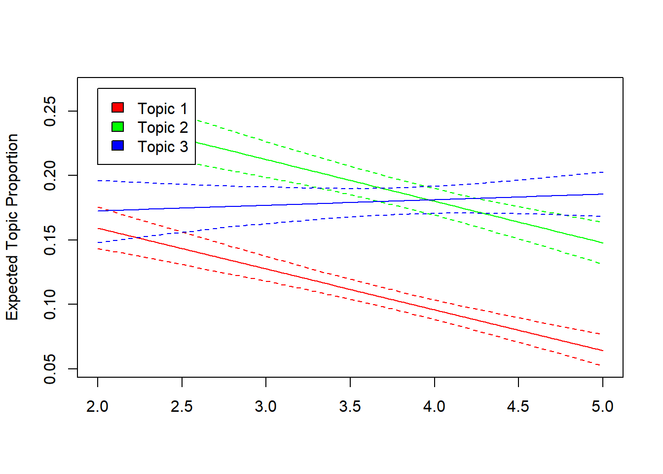

It seems that topic 1 and 2 became less prevalent over time. For these topics, time has a negative influence. However, there is no consistent trend for topic 3 - i.e., there is no consistent linear association between the month of publication and the prevalence of topic 3.

A next step would then be to validate the topics, for instance via comparison to a manual gold standard - something we will discuss in the next tutorial.

13.6 Take Aways

Vocabulary:

Topic Modeling: Form of unsupervised machine learning method used to exploratively identify topics in a corpus. Often, these are so-called mixed-membership models.
K: Number of topics to be calculated for a given a topic model.
Word-Topic-Matrix: Matrix describing the conditional probability with which a feature is prevalent in a given topic.
Document-Topic-Matrix: Matrix describing the conditional probability with which a topic is prevalent in a given document.

Commands:

Running a structural topic model: convert(), stm
Find a suitable number of topics based on statistical fit: searchK()
Inspect result of a structural topic model: plot(), labelTopics(), make.dt(), findThoughts(), estimateEffect()

13.7 More tutorials on this

You still have questions? The following tutorials & papers can help you with that:

13.8 Test your knowledge

You’ve worked through all the material of Tutorial 13? Let’s see it - the following tasks will test your knowledge.

13.8.1 Task 13.1

Using the dfm we just created, run a model with K = 20 topics including the publication month as an independent variable.

Is there a topic in the immigration corpus that deals with racism in the UK?

If yes: Which topic(s) - and how did you come to that conclusion?

Let’s keep going: Tutorial 14: Validating automated content analyses.

In most cases, the answer is: No.↩︎