10 Tutorial 10: Reading text into R & important data types
After working through Tutorial 10, you’ll…
- know how to read text files and data into R
- know about data types often used for handling textual data in R
10.1 Reading text into R & encoding issues
As an example, please download the two text files for Tutorial 10 from OLAT (via: Materials / Data for R). These files are two fictional news articles, as you’ll see (titled: “text1_tutorial10” and “text2_tutorial10”)
To read these texts into R, we will use the readtext package.
Here, we tell R to read in all files from our working directory that have a .txt extension.
The asterisk * indicates that the file name can contain any characters before the .txt. ending (note that we are once again working with regular expressions here).
In other words: R should read in all files in the working directory that are saved as “.txt” files.
library("readtext")
texts <- readtext("*.txt")Important: Pay attention to the character encoding of texts when reading them in.
Character encodings:
Computers store individual characters - such as the letters “w”, “o”, “r”, and “d”, which stand for “word” - using a specific numeric code (bytes) assigned to each character. For example, “word” is stored as “01110111 01101111 01110010 01100100”.
By using a specific character encoding, R determines which numeric 0/1 code is associated with which character (for instance, which number is translated to which letter when translating bytes to character data).
In a sencse, character encodings are the “key”, with which the computer determines how to translate numeric 0/1 to a character format.
The problem: Different encodings coexist.
As you know, many languages contain special characters - in German, for example, the letters “ü” and “ä” (which are not part of the English-language alphabet, for instance). These special characters are often read in incorrectly by the computer if the computer is not told to use the correct specific character encoding. If the computer uses its default encoding, these special characters may be “translated” incorrectly.
An example: The German news brands “Süddeutsche Zeitung” contains the special character “ü”, which is often read in incorrectly by R given that it is not part of many languages/encodings.
We assign the word Süddeutsche Zeitung to the object word and ask R which encoding word has:
word <- "Süddeutsche Zeitung"
Encoding(word)
## [1] "latin1"As you see, the correct encoding here is latin1. See what happens if we change the encoding, for instance to the default encoding of many computers, “UTF-8”?
The consequence: R has the wrong “key” (i.e., encoding) to return the correct result:
Encoding(word) <- "UTF-8"
word
## [1] "S<fc>ddeutsche Zeitung"Please note that your computer’s default encoding may be different from mine, which is why you may get different results here (and when reading in example texts for this tutorial):
Sys.getlocale(category = "LC_CTYPE")## [1] "English_United States.1252"When reading texts into R, you can use readtext to specify which encoding should be used.
Oftentimes, R recognizes the correct encoding on its own. Since I did not encounter any problems with encodings, I set the encoding to the default value NULL.
However, you could specify another encoding if you encounter problems (or - otherwise - solve encoding problems by manipulating texts afterwards).
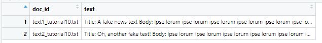
texts <- readtext("*.txt", encoding = NULL)Checking the results, we see that R has read in a data frame:
- doc_id: contains the titles of all “txt”.files
- text: contains the text of all “txt”.files
View(texts)Image: Texts read in by R
Apart from the data frame format (which you already know!), there are some more specific types of objects you will encounter when working with text data. We’ll get to these now.
10.2 Data types
The following types of objects are important for working with textual content in R:
- Data frame objects
- Corpus objects
- Token objects
- Document-feature-matrices (DFMs)
For illustration, we’ll work with a text corpus already included in the R-Package Quanteda-Corpora-Package. This package is still in development status, i.e. not yet officially published on CRAN. You can access it via the developer platform Github. For simplicity, I have downloaded the corpus already read it into an R environment (with some minor specifications).
You can find the corresponding R file in OLAT (via: Materials / Data for R) with the name immigration_news.rda.
These files are news articles from the UK reporting on the topic of immigration from 2014. The data is in a similar format as you would get if you read their text with the readtext package.
Source of the data set: Nulty, P. & Poletti, M. (2014). “The Immigration Issue in the UK in the 2014 EU Elections: Text Mining the Public Debate.” Presentation at LSE Text Mining Conference 2014. Accessed via the quanteda corpus package.
load("immigration_news.rda")10.2.1 Data frames
The readtext package stores your texts in a data frame, which consists of as many rows as texts and two columns, namely doc_id and text.
str(data)## 'data.frame': 2833 obs. of 2 variables:
## $ doc_id: chr "text1" "text2" "text3" "text4" ...
## $ text : chr "support for ukip continues to grow in the labour heartlands and miliband should be scared\nby leo mckinstry \"| __truncated__ " \nnews\n30 lawless migrants try to reach uk each night\ngiles sheldrick \n402 words\n14 april 2014\nthe dai"| __truncated__ " \nnews\n30 lawless migrants try to reach uk each night\ngiles sheldrick \n610 words\n14 april 2014\nthe dai"| __truncated__ " \nnews\n£10m benefits scandal\nmartyn brown \n151 words\n14 april 2014\nthe daily express\ntheexp\n1 nation"| __truncated__ ...If you want to read a single text, you can access it via indexing. As an example, let’s take a look at text number 100:
data$text[100]## [1] "nick cleggs blunt solution to knife crime\nby nick ferrari \n1304 words\n11 may 2014\n0100\nexpresscouk\nexco\nenglish\ncopyright 2014 \nit is very easy to have a go at deputy prime minister nick clegg\nindeed last week the labour party bizarrely decided to devote its entire party political broadcast to belittling him seeking to portray him as a bullied put upon wimp who is routinely ignored by coalition cabinet colleagues\nnever mind that top of most sane people's worry list is the economy jobs immigration national security or the state of the health service labour lavished a considerable sum to send up nick clegg in a film that was humourless pointless and left most people feeling they could not care less\nas someone in the media who probably knows mr clegg as well as anyone i can assure you he is too robust and steadfast for this to have fazed him for even a heartbeat\nhowever what desperately does require more scrutiny is his avowed intent to block conservative plans for a crackdown on knife crime\nthis was promised in david cameron's manifesto in 2010 but was another victim of the fact that the tories managed to blast the ball over the bar in front of the empty goal of that general election and needed a coalition with the lib dems to get into power\nin truth the commentators and political chatterati have been deeply dismayed by how little the coalition has fought and how well in most areas it has performed\nhence they seize on any bit of discord and treat it as if it were fisticuffs across the cabinet table\nthis bold stance by clegg could be the one however that causes a good old-fashioned rumpus and possibly demonstrates that despite taking all the calls we have done together down the months he might not always have been listening\npartly spurred on by the stabbing to death of a teacher in her classroom the conservatives want to introduce automatic jail terms for repeat knife offenders a \"two strikes and you're in\" kind of policy but clegg is adamantly against it\nhe dismisses it as an attempt to introduce \"headline-grabbing solutions\" in the wake of the killing of ann maguire\nhe goes on to claim it could \"turn the young offenders of today into the hardened criminals of tomorrow\" and calls it \"a backwards step that will undermine the government's rehabilitation revolution\"\nthis is high stakes stuff for mr clegg and if as is being mooted the labour party opts to support the conservatives at a time when the lib dems' poll ratings are bouncing on the bottom and in one case they are being beaten even by the green party clegg's party risks being stranded on a political peninsula\nclegg is a shrewd strategist and is that rare politician who usually actually stands by his beliefs however unpopular they might be\nas the calls came in last week he did not move an inch on his trenchant opposition"10.2.2 Corpus
A second object type you will encounter is a corpus.
The corpus object is similar to a data frame: Each row contains a unique text and each column contains variables for each text (for instance the name of the respective text).
You may wonder: Why do we need corpus objects when we already have similar information when using the data frame format?
Quite simply: Because there are many useful functions in the quanteda package (such as making R return individual sentences as our unit of analysis rather than whole texts) that cannot be applied directly to a data frame object.
You can create a corpus object by activating the quanteda package and then using the corpus command.
Let’s transform our texts to a corpus and get some basic information on it:
install.packages("quanteda")library("quanteda")
corpus <- corpus(data)
print(corpus)## Corpus consisting of 2,833 documents.
## text1 :
## "support for ukip continues to grow in the labour heartlands ..."
##
## text2 :
## " news 30 lawless migrants try to reach uk each night giles..."
##
## text3 :
## " news 30 lawless migrants try to reach uk each night giles..."
##
## text4 :
## " news £10m benefits scandal martyn brown 151 words 14 a..."
##
## text5 :
## " news taxpayers £150m bill to oust illegal immigrants gile..."
##
## text6 :
## " news un expert hits at boys club sexism in britain helene..."
##
## [ reached max_ndoc ... 2,827 more documents ]As indicated by the result, the corpus contains 2,833 documents - which is not surprising, because this is exactly the number of rows our data frame data contained.
An additional advantage of a corpus object is that you can store document-level variables for individual texts to later use them for analysis.
For example, the data frame data contained the names of our texts in the doc_id column:
head(data$doc_id)## [1] "text1" "text2" "text3" "text4" "text5" "text6"To assign the value of the variable data$doc_id to the correct text in corpus, we rely on document-level variables and assign these via docvar():
corpus <- corpus(data$text , docvars = data.frame(ID = data$doc_id))
head(docvars(corpus))
## ID
## 1 text1
## 2 text2
## 3 text3
## 4 text4
## 5 text5
## 6 text6A common example of a document-level variable we may need is the publication date of an article.
The problem: We don’t have any information on the publication date of each article yet. How do we get this information?
Since we know that our texts have all been published in 2014 (as indicated by the data source from which the texts stem), we can already assign the year 2014 as document-level variable:
corpus <- corpus(data$text,docvars = data.frame(ID = data$doc_id, year = rep("2014", nrow(data))))
head(docvars(corpus))
## ID year
## 1 text1 2014
## 2 text2 2014
## 3 text3 2014
## 4 text4 2014
## 5 text5 2014
## 6 text6 2014But how do we get any information on the month in which an article was published?
Let’s take a closer look at our texts using two examples:
data$text[1000]## [1] " \nfrontpage\nshould nigel farage have stuck to his guns newark might just have voted him in\njonathan brown \n725 words\n1 may 2014\n1002\nindependent online\nindop\nenglish\n© 2014 independent print ltd all rights reserved \nnigel farage will never know whether newark was set to join the ranks of bermondsey hamilton or bradford west in the political atlas of great by-election upsets\nyet if the mood in the nottinghamshire town's georgian market place was anything to go by yesterday the decision not to contest the vacant seat could go down as one of missed opportunity rather than inspired tactical retreat\nbutcher michael thorne 48 was an unabashed fan of mr farage having spent 15 minutes in the ukip leader's company at a recent market day\n\"he is a down-to-earth bloke and he doesn't beat around the bush it's about time we had someone like that\" he said \"it's about british people for british jobs as far as i'm concerned we need to support as many local people as we can\" he added\ncustomer terence dilger 65 was pondering what to have for his dinner he was less equivocal in voicing his support for mr farage\n\"i think he is right on immigration - it is as simple as that\" he said \"when i first came to newark it was an ordinary town now it is a league of nations you feel like a stranger in your own town even if he didn't win he would have got his message across\"\naccording to the 2011 census figures newark and neighbouring sherwood remain remarkably homogenous from a population of 114000 some 94 per cent describe themselves as white british the number of residents from eu accession states was just 18 per cent - just over 2000 people and lower than the english average but that is not the perception\napril 2014 a month of ukip gaffes and controversies\nshopper yvonne mastin 61 was happy to repeat one of ukip's slogans she had read on a leaflet recently put through her door \"we do want britain back to how it used to be it's got totally out of hand\" she said \"i believe in immigration if they have got something to bring\" she said\nover at his stall selling mobility scooters was kevin walker 54 also a farage fan \"a vote for him is a vote not for the other two\" he said \"there are too many of them [immigrants] whoever said they are not taking our jobs is talking rubbish if you go to the fields around here see how many of them speak english\n\"it's the same anywhere you go now i do a lot of care homes and they are all foreign staff it's not because we won't do the jobs it's because they won't kick up a fuss and they are cheaper they will work long hours but it is not right\" he added\nukip is currently looking for a candidate to stand in the seat in which it came fourth with just 38 per cent of the vote in 2010\nthe conservatives have selected robert jenrick - international business director at christie's - i"data$text[2000]## [1] " \nexpats wish you lived here\nby christopher middleton \n1727 words\n26 april 2014\n0810\nthe telegraph online\nteluk\nenglish\nthe telegraph online © 2014 telegraph media group ltd \nas more brits bid adios to spain we seek new destinations for the expat dream\nfor us brits it's been the equivalent of a property dunkirk for years we have been happily sending out thousands of citizens to start a new life in spain - about 760000 sun-seekers have moved there since 1995 all of a sudden though the economic sun has gone behind the clouds and our bucket-and-spade brigades are withdrawing at an alarming rate according to official figures some 90000 of us have forsaken the costas and returned to these shores\nthe news has sent the nation rushing to our atlases to seek out new spots in which to settle it's estimated that between 45 and 47 million british citizens live abroad for at least part of the year\nquestion is when the world is your oyster how do you find a place to live that is a genuine pearl here are some suggestions…\naustralia\nestimated number of expat brits 11 to 12 million\nmost popular areas sydney melbourne perth\nproperty prices in sydney you pay £550000 for a three-bed hou>se in perth you pay the same for a four-bed house with sea views\nflight time to uk 20 hrs 45mins from sydney\nclimate sydney averages 26c 78f and 16c 60f in summer and winter perth 31c 87f and 18c 64f\ncost of a pint of beer 65 australian dollars £360\ncost of restaurant meal 40 australian dollars £22\nthe good points australia tops the natwest international personal banking quality of life survey it's been in the top three since 2009 you'll still get your uk pension too albeit frozen from when you arrive\nnot-so-good points more british expats than any other country in the world\nwhat you'd miss about the uk understatement\nunited states of america\nestimated expat brits 829000\nmost popular areas there's a smattering of us in the big cities but we're at our most concentrated in florida one study says more brits migrate to the us than from any other nation legally that is\nproperty prices in florida you can get a humble one-bed condominium apartment for £25-£40000 or an up-market four-bedroom villa for under £250000\nflight time to uk 11 hours from the west coast seven hours from the east\nclimate average minimum 167c 62f average maximum 28c 82f orlando has 107 days per year where temperatures are 32c 89f or more\ncost of a pint of beer $382 £227\ncost of restaurant meal $30 £17\nthe good points big portions big country year-round warmth that's why they call florida the sunshine state - or is it the orange juice state\nnot-so-good points if you're working you get very little holiday per year nine-10 days and the cost of health insurance is enough to make you feel quite ill\nwhat you'd miss pessimism\ncanada\nestimated expat br"We see that each text contains its publication date after its title and the number of words at the beginning of each text.
We’ll ignore the strange string //n here for now - I’ll explain what this string pattern stands for at a later point in time.
- Text number 1000 seems to have been published on May 1 since the text contains the following text string: “1 may 2014”.
- Text number 2000 seems to have been published on April 26 since the text contains the following text string: “26 april 2014”.
How can we now systematically identify the publication month for each individual text and store it as a document-level variable?
Solution: We use the str_extract() function (you already know this function!)
The str_extract() function only reads the first match of a pattern to ensure that other matches are not returned.
Since the publication month is always mentioned at the beginning of each article, reading in any more subsequent matches is likely to introduce noise. That is why we do not use, for instance, str_extract_all().
Now we need to write a pattern that correctly identifies an article’s publication month.
Solution:
We remember: In each text, the article’s publication month is given in a format similar to this: “1 may 2014”.
Our search pattern thus needs to be flexible enough to:
- Finds the words “january” or “february” or “march” or “april” or “may” or “june” or “july” or “august” or “september” or “october” or “november” or “december” in the text.
- However, these pattern should only be matched if they occur after any two digit number and before the string 2014.
Why?
Since we now know that the publication month of the article is always mentioned after the day of publication, i.e., any one to two digit number (see “1 may 2014”), and before the publication year, i.e., 2014 (see “1 may 2014”), we can use these two strings to ensure that R only identified months if they are mentioned in this format.
Theoretically, months could also be mentioned in the text of an article where they do, in fact, not indicate the publication month of the article.
For example, an article may contain the following sentence: “The financial crisis is going to hit in December”. We don’t want R to retrieve the pattern “december” and mistakenly use this string as the month the article was published.
A pattern that returns any month (written as january, february, march, etc.) that occurs after the string any one to two digit number and before the string 2014 looks like this:
data$month <- str_extract(string = data$text,
  pattern = "[0-9]+ (january|february|march|april|may|june|july|
  august|september|october|november|december) 2014")
What does this pattern entail?
- [0-9]+: We tell R to search for any numbers from 0-9, [0-9], which should occur at least once, but can occur more often, using the quantifier +. For example, the publication date could be 1 May (one number) as well as 22 May (two numbers).
- " ": This string pattern should be followed by a blank space.
- (january|february|march|april|may|june|july|august|september|october|november|december): This string pattern should be followed by the word january or the word february or the word march or the word april or the word may or the word june or the word july or the word august or the word september or the word october or the word november or the word december.
- " ": This string pattern should be followed by a space.
- 2014: This string pattern should be followed by the string pattern 2014.
This seems to have worked: Our code correctly identified each article’s publication month.
However, the vector data$month now contains a lot of additional information that we don’t need (for instance the day or the year of an article’s publication).
data$month[1]## [1] "10 april 2014"next, we only keep those string patterns out of data$month that actually represent the month:
data$month <- str_extract(string = data$month,
  pattern = "january|february|march|april|may|june|july|
  august|september|october|november|december")
data$month[1]
## [1] "april"Using the table() command, we can now get an overview of the months within which our articles were published:
table(data$month)##
## april february march may
## 835 252 933 813To later use this information for analysis, we assign data$month to corpus as a document level variable:
corpus <- corpus(data$text,
                 docvars = data.frame(ID = data$doc_id,
                                      year = rep("2014", nrow(data)), month = data$month))
head(docvars(corpus))
## ID year month
## 1 text1 2014 april
## 2 text2 2014 april
## 3 text3 2014 april
## 4 text4 2014 april
## 5 text5 2014 april
## 6 text6 2014 aprilFor R to return relevant info - for instance these document level variables - for a small number of documents, we can use the following command:
summary(corpus[1:5])## Corpus consisting of 5 documents, showing 5 documents:
##
## Text Types Tokens Sentences ID year month
## text1 266 449 1 text1 2014 april
## text2 245 414 1 text2 2014 april
## text3 295 516 1 text3 2014 april
## text4 120 170 1 text4 2014 april
## text5 293 480 1 text5 2014 aprilThe summary command gives some more useful info about our corpus: Not only do we now know that the first five texts were all published in April. The summary command also tells us how many types, tokens and sentences each document contains:
- Types: denote the number of distinct features, i.e., the number of distinct words.
- Tokens: denote the number of all features, i.e. the number of all words.
- Sentences: denote the number of all sentences.
A short info here: Since the data set immigration_news.rda does not contain any punctuation marks - e.g. all points have been removed - and quanteda calculates the number of sentences using, among other things, punctuation marks (sentences are identified by string patterns ending on a punctuation mark), this information is certainly not correct. Ignore it for now.
What are types and what are tokens? And what do we need them for?
That’s what we’re learning now:
10.2.3 Tokenization, Tokens & Types
As you already know, we often break texts to individual features in a bag-of-word approach. This process of converting whole texts into individual features is called tokenization and allows us to process texts automatically.
Features can be individual words, word chains, entire sentences, numbers, or punctuation marks.
In R, this tokenization is done with tokens().
Here, we specify that we want our corpus to be broken down to single texts not, for example, sentences.
tokens <- tokens(corpus, what = "word")This is how the first document of our corpus looks like after tokenization:
tokens[1]## Tokens consisting of 1 document and 3 docvars.
## text1 :
## [1] "support" "for" "ukip" "continues" "to" "grow" "in" "the"
## [9] "labour" "heartlands" "and" "miliband"
## [ ... and 437 more ]I want you to understand the difference between types and tokens based on a simple example:
sentence <- "After this tutorial, I will certainly need a break. I will likely need to go for a walk."
#Number of tokens
ntoken(sentence)
## text1
## 21#Number of types
ntype(sentence)## text1
## 16The sentence “After this tutorial, I will certainty need a break. I will likely need to go for a walk.” consists of 21 tokens (i.e., a total of 21 features) and 16 types (i.e., of these 21 features, 16 features are different).
Why are these numbers different?
The features “a”, “I”, “will”, “need” and the point “.” occur twice in the sentence. Correspondingly, they are considered as 10 tokens, but only as 5 distinct types.
10.2.4 Document-Feature-Matrix
In many cases, we are interested in finding overarching similarities and differences across documents:
- Which features occur across different documents?
- How are documents similar or different based on their feature occurrences?
To answer these questions, we use what is called a document-feature-matrix (DFM).
A document-feature-matrix is a matrix in which:
- rows denote the documents that our corpus contains
- columns denote the features that occur across all documents
- cells indicate the frequency of a single feature in a single text
Using the DFM, we can identify similarities or differences between feature occurrences across texts.
dfm <- dfm(tokens)
print(dfm)
## Document-feature matrix of: 2,833 documents, 41,995 features (99.42% sparse) and 3 docvars.
## features
## docs support for ukip continues to grow in the labour heartlands
## text1 2 5 7 1 5 1 17 28 8 2
## text2 0 1 1 0 19 0 9 26 0 0
## text3 0 1 1 0 22 0 10 28 0 0
## text4 0 4 0 0 3 0 2 8 0 0
## text5 0 9 1 0 8 0 11 17 0 0
## text6 0 1 0 0 4 0 8 11 0 0
## [ reached max_ndoc ... 2,827 more documents, reached max_nfeat ... 41,985 more features ]By inspecting the output, we learn that…
Our corpus consists of 2,833 documents. The first line of the DFM describes the first document, the second the second document, and so on.
We have 41,995 features occurring across all 2,833 documents. These features denote types, i.e., different features that occur. In our case, we used tokenization to break our texts down to words. Here, our entire corpus contains 41,995 words. The first column of the DFM describes the first feature: the word support.
Cells describe how many times each feature occurs in each document. For example, the feature support occurs twice in the first article, but never in articles 2-6. This indicates that the feature support does not occur in all documents - in difference to the feature “the”, for instance (displayed in column 8), which occurs in all documents, some of them very frequently.
In addition, R tells us that our DFM is 99.4% “spare”. What does this mean? Sparsity can be understood as the number of cells that contain a 0: 99.4% of our cells contain a 0. This is not surprising - while words like “the” or “to” occur in many texts, this will not necessarily be the case for many other words like “support” or “continues”. Many features occur in very few texts, while some features (the, and, or) occur in almost all texts. As such, our DFM probably includes some features that are not very informative.
We can use the DFM to analyze which words are most frequent:
topfeatures(dfm, 20)## the to of a and in that is for on it he was by as with are be from "
## 69066 34040 30360 27229 25144 22655 13396 12510 11042 9630 8257 8162 7997 7538 7530 6769 6469 6137 5975 5966Here, we can already see that the top features are not very informative. The most common features are classic stop words, i.e. words that have little value for understanding the content of our corpus: the, to, of, a, or and.
If we only look at the most frequent words, we would not get a sense of what the texts in our corpus are dealing with. Furthermore, we see that R has stored punctuation marks - here quotation marks - as words (last top feature). In some cases, such punctuation may not be too helpful for understanding the content of corpus.
In order to reduce our texts to informative features, i.e., those features that are helpful for finding similarities and differences between texts, we have to do some preprocessings. This also has the advantage of (hopefully) reducing the amount of sparse data and speeding up analysis.
How to do such preprocessing is exactly what the next tutorial deals with.
10.3 Take Aways
Vocabulary:
- Character encoding: Character encoding refers to the “key” with which the computer determines how to translate characters into bytes (as numeric information) - and vice versa.
- A corpus is like a data frame. As rows, it contains the articles of your corpus, i.e. individual texts, and as columns the corresponding document-level variables, for instance an article’s publication date.
- Tokenization is the process of breaking down articles to individual features, for instance words.
- Features are the result of such tokenization, often individual words in bag-of-word approaches.
- Tokens denote all the features that a text/corpus contains.
- Types denote all the different features that a text/corpus contains.
- A document-feature-matrix is a matrix where rows identify the articles of your corpus and columns its features. Each cell indicates how often a feature occurs in a particular article.
Commands:
- Reading in text files: readtext()
- Creating a corpus: corpus(), docvars()
- Tokenization: tokens()
- Creating a Document-Feature-Matrix: dfm()
10.4 More tutorials on this
You still have questions? The following tutorials & papers can help you with that:
- Quanteda Tutorials by Watanabe, K., & Müller, S, Tutorial “Data Import” und “Basic Operations”
- Automated Content Analysis with R by Puschmann, C., & Haim, M., Tutorial “Basics”
Let’s keep going: with Tutorial 11: Preprocessing