Chapter 5 Scale

Scale（刻度尺）: 指觀測值對應到美感呈現(aes mapping)的對應方式。

不同aes的對應方式有不同可能設定：

scale_x, scale_y
- scale_color
- scale_linetype
- 參考不同geom使用說明裡的Aesthetics部份，查詢所用的geom有那些aes mapping。接著到scale說明查詢scale詳細說明。

5.1 層疊

以層疊方式在欲設定的geom之後疊加上去。

範例

library(ggplot2)
library(dplyr)
library(showtext)
font_add("QYuan","cwTeXQYuan-Medium.ttf") # 新增字體
showtext_auto(enable=TRUE)
theme_set(theme_classic())

mpg %>% ggplot(aes(x=cty,y=hwy,color=class))+
  geom_point()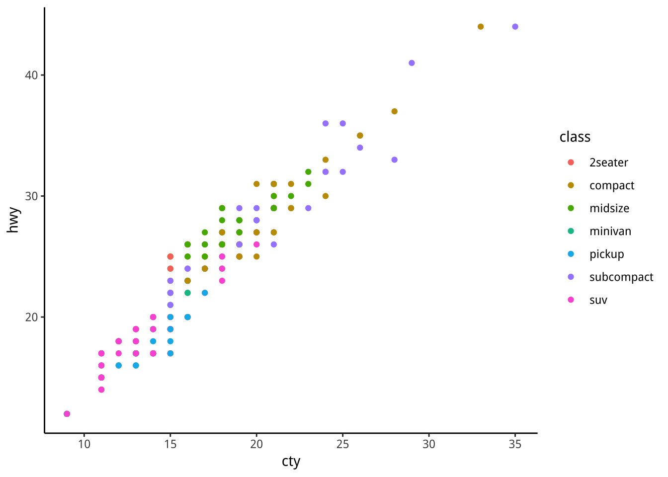

mpg %>% ggplot(aes(x=cty,y=hwy,color=class))+
  geom_point() -> f1

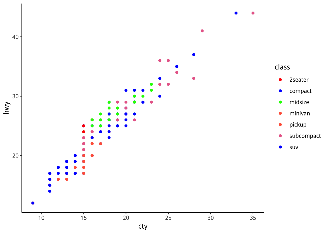
f1+
  scale_color_manual(
    values=c("red","blue","green","tomato","tomato","#e86b97","blue")
  )

f1+scale_color_brewer()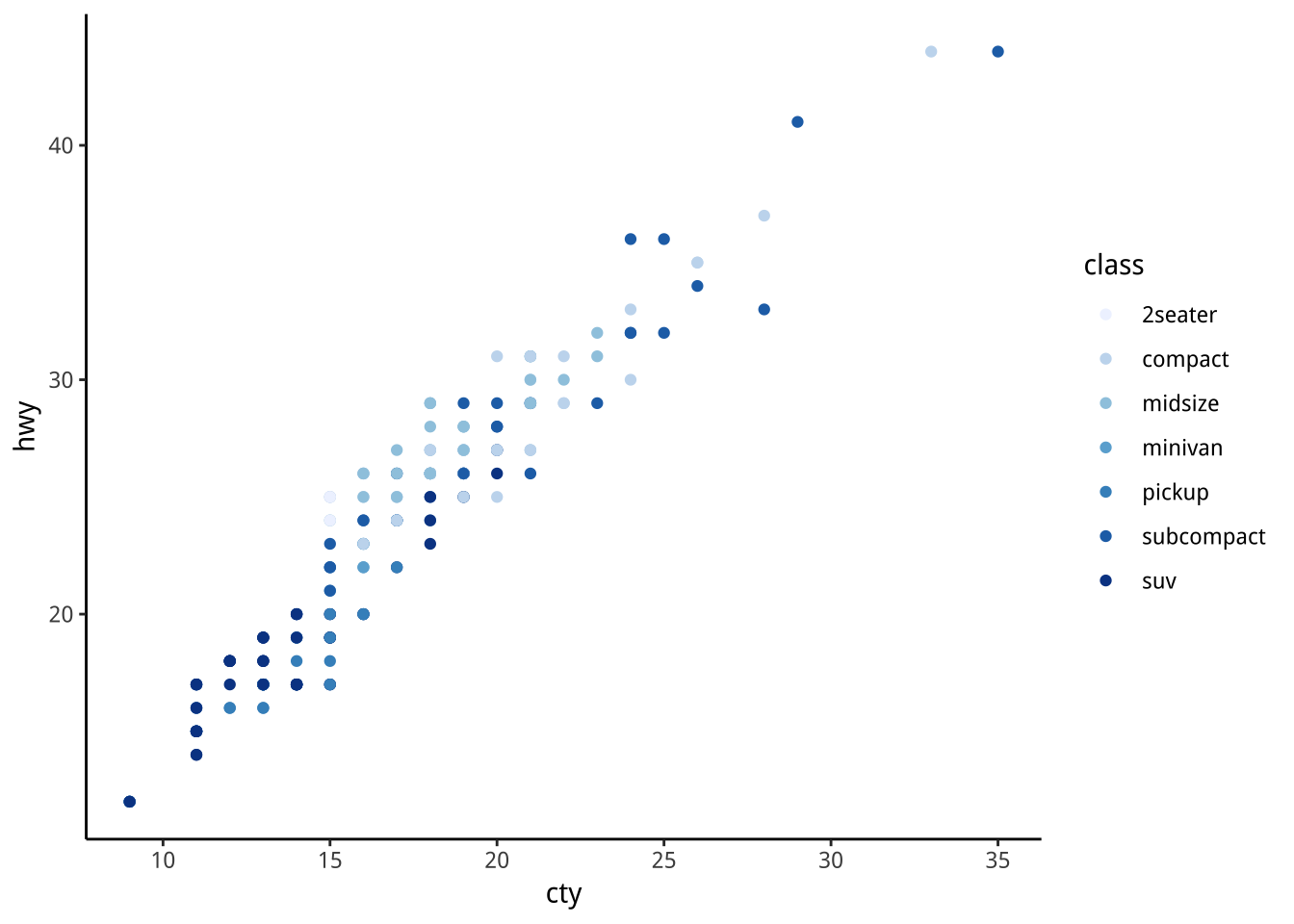

5.2 Color

5.2.1 參考資料

Cookbook for R: Graph colors

若要更改color美感呈現，可使用scale_color_*，其中*有多種資料對應顏色的方式可選，如

scale_color_hue
- scale_color_brewer
- scale_color_distiller, 等等。

每一種詳細用法可參見Scales reference。

用英式拼法colour或美式拼法color都可以。

5.2.2 間斷變數(Dicrete variable)

scale_color_

hue
brewer
scale_color_manual: 自訂調色盤(Palette)

5.2.2.1 hue: 內定選色方式

By default, the colors for discrete scales are evenly spaced around a HSL color circle. For example, if there are two colors, then they will be selected from opposite points on the circle; if there are three colors, they will be 120° apart on the color circle; and so on.

The colors used for different numbers of levels are shown here:

1st row: 1 level 2nd row: 2 levels so on….

The default color selection uses scale_fill_hue() and scale_colour_hue().

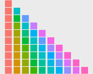
colorselect

5.2.2.2 brewer

The brewer scales provides sequential（強調順序）, diverging （強調離異）and qualitative（強調不同屬性） colour schemes from ColorBrewer. These are particularly well suited to display discrete values on a map. See http://colorbrewer2.org for more information.

5.2.2.2.1 強調不同屬性(Qualitative)

type="qual"

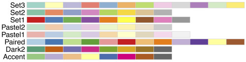
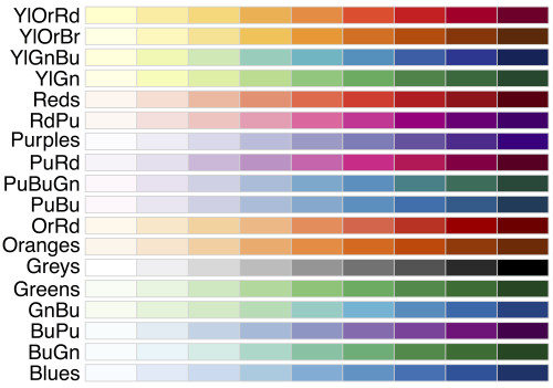
5.2.2.2.2 強調順序(Sequential)

type="seq"

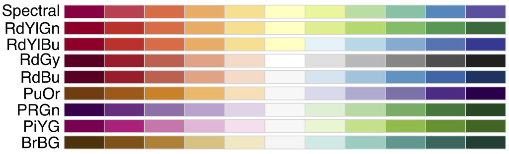
5.2.2.2.3 強調離異(Diverging)

type="div"

5.2.2.3 manual

顏色可用hex code去查詢。

Hexadecimal color code

Colors can specified as a hexadecimal RGB triplet, such as “#0066CC”. The first two digits are the level of red, the next two green, and the last two blue. The value for each ranges from 00 to FF in hexadecimal (十六進位：0-9,A-F) notation, which is equivalent to 0 and 255 in base-10. For example, in the table below, “#FFFFFF” is white and “#990000” is a deep red.

cbPalette <- c("#999999", "#E69F00", "#56B4E9", "#009E73", "#F0E442", "#0072B2", "#D55E00", "#CC79A7")

# The palette with black:
cbbPalette <- c("#000000", "#E69F00", "#56B4E9", "#009E73", "#F0E442", "#0072B2", "#D55E00", "#CC79A7")

# To use for line and point colors, add
  scale_colour_manual(values=cbPalette)

5.2.3 連續變數(Continuous)

scale_color_

continuous: 內定使用gradient。
gradient: 自定色階變化。
distiller: 利用brewer再去連續平滑色度變化。

5.2.3.1 gradient

範例

Color Chart

df <- data.frame(
  x = runif(100),
  y = runif(100),
  z1 = rnorm(100),
  z2 = abs(rnorm(100))
)

# Default colour scale colours from light blue to dark blue
ggplot(df, aes(x, y)) +
  geom_point(aes(colour = z2)) -> gradientBase
gradientBase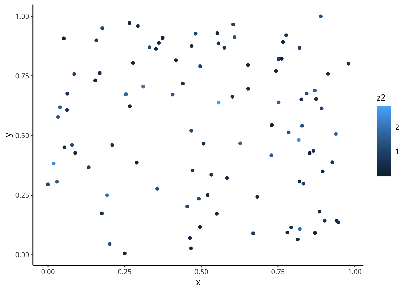

5.2.3.1.1 sequential

gradientBase+scale_color_gradient(low="#66FFFF",high="#6600FF")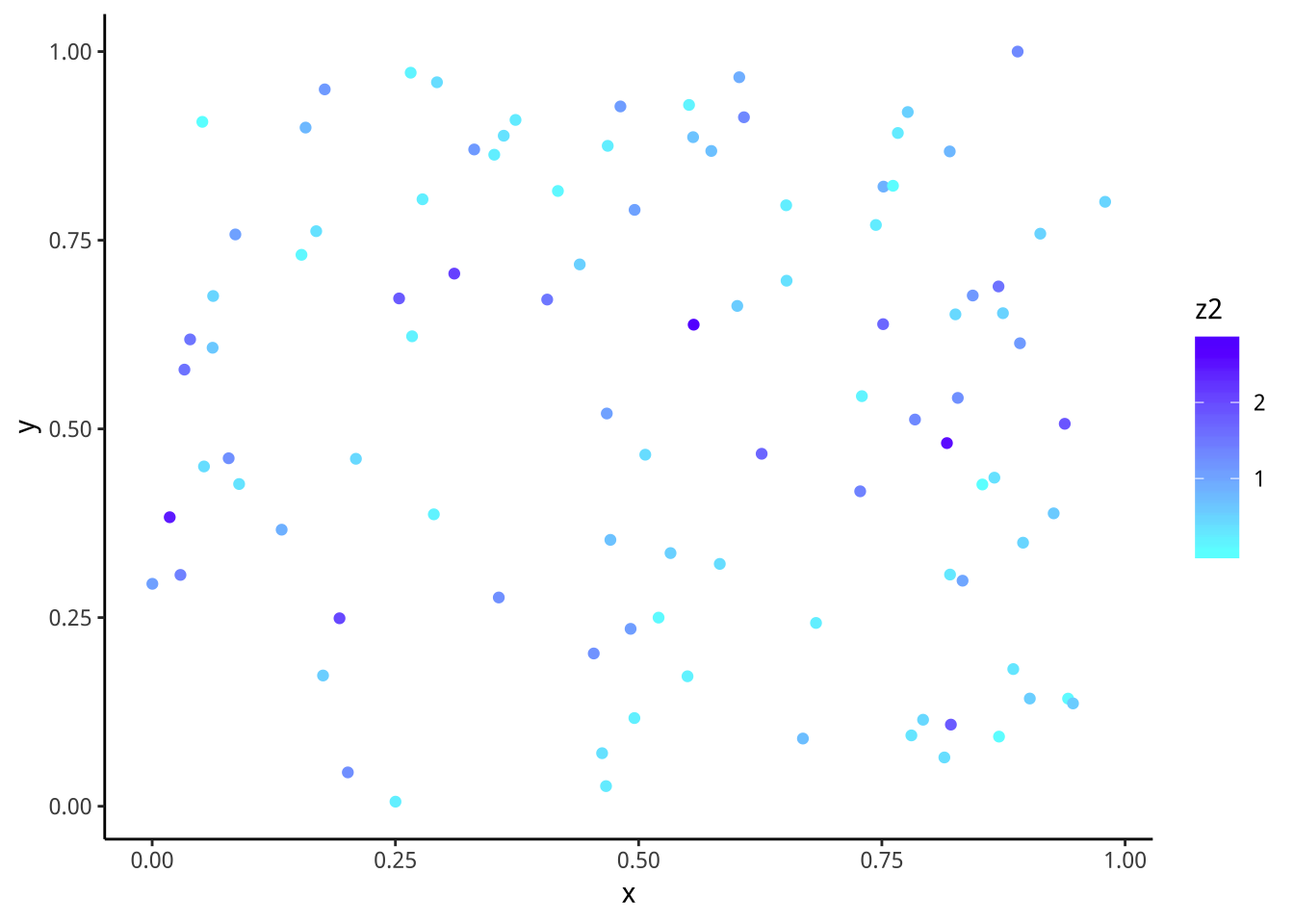

5.2.3.1.2 diverging

使用內定色。

gradientBase+scale_colour_gradient2(midpoint = 1.5)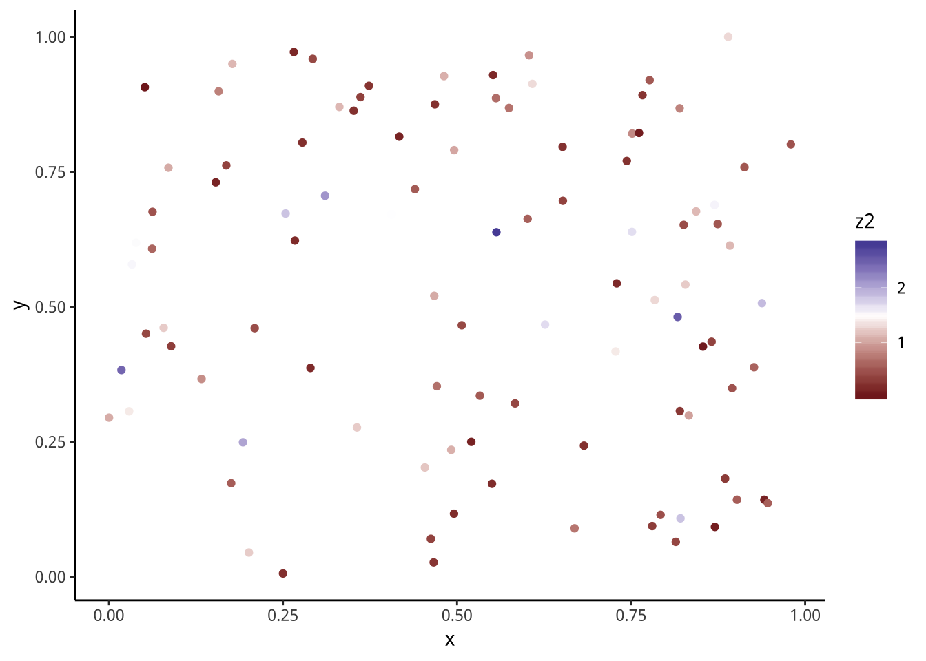

gradient2內定使用不刺眼的muted red與muted blue. 下面的code可以顯現兩者的差別。另外，由於mute的效果是由alpha來進一步達成，所以會看到ARGB的8碼Hex code。

library(scales)
show_col(c("red", "blue", muted("red"), muted("blue")))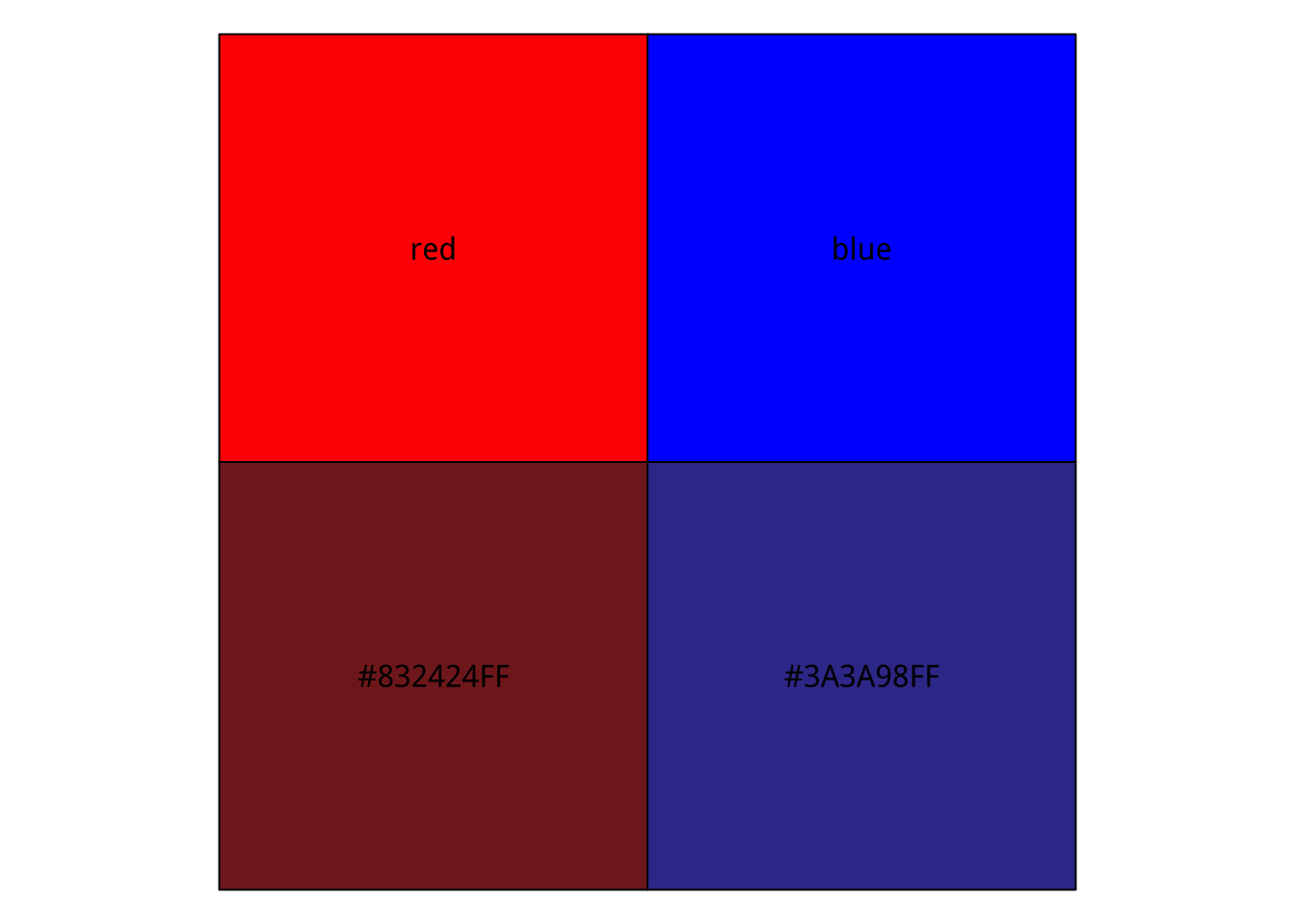

自定顏色。

show_col(c("#704a6c","#f58220"))

gradientBase+scale_color_gradient2(
  low="#f58220",
  high="#704a6c",
  midpoint = 1.5)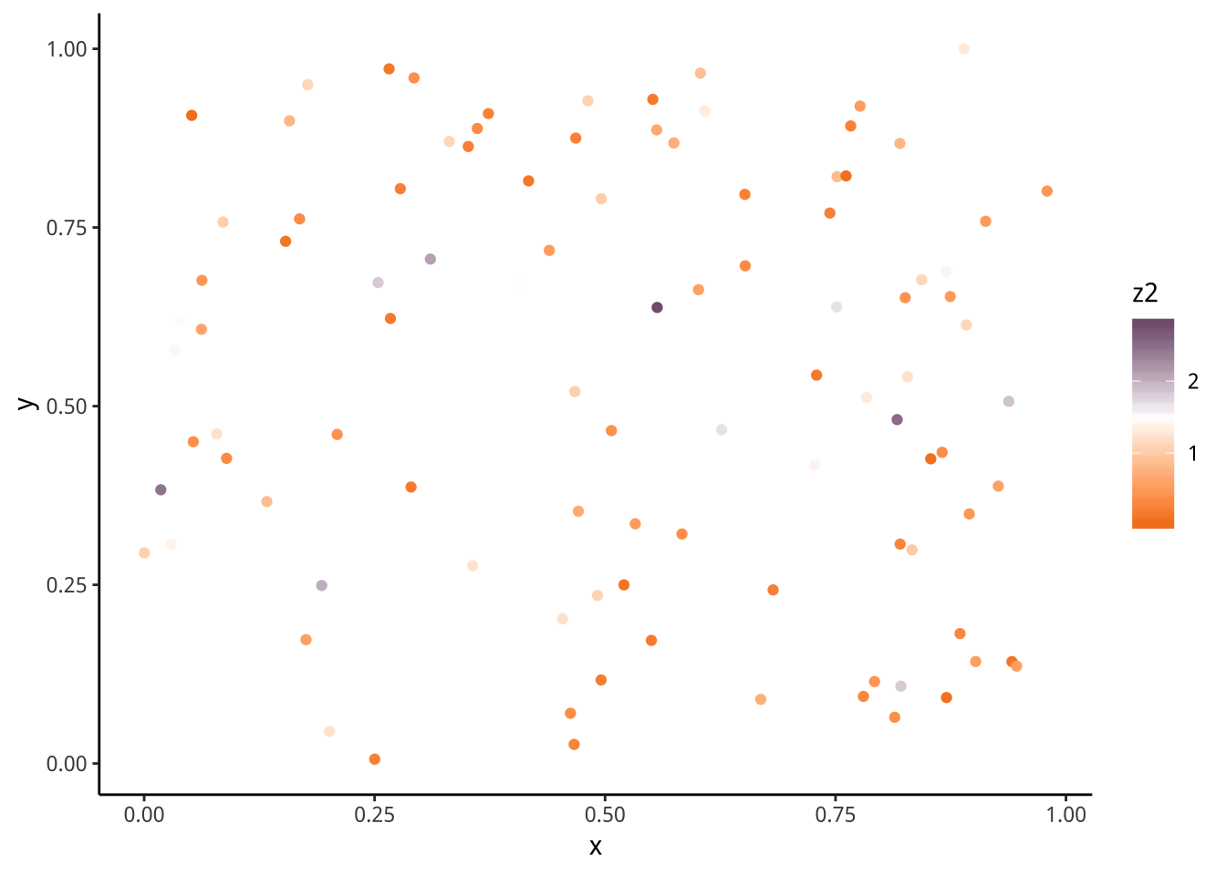

5.2.3.2 distiller

範例

5.2.3.2.1 sequential

gradientBase+scale_color_distiller()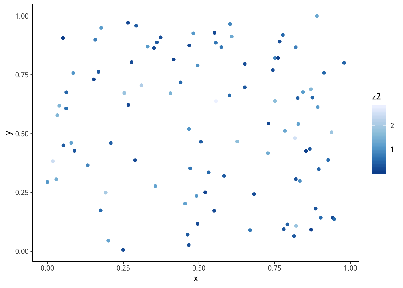

5.2.3.2.2 diverging

gradientBase+scale_color_distiller(type="div")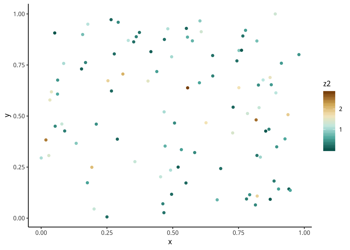

5.2.4 其他色彩名詞

Hue（色相）、Chroma（飽和度）、luminance（亮度）

5.3 其他參考資料

色盲友善的scale_color_viridis

Make your own color palettes with paletti

5.4 練習

執行以下程式產生各家銀行的三個月、一年期定存固定利率及其利差。

library(readr)
InterestRateData <- read_csv("https://raw.githubusercontent.com/tpemartin/github-data/master/InterestRateData.csv")

# 取出變數
InterestRateData %>% select(
  銀行,
  年月,
  `定存利率-三個月-固定`,
  `定存利率-一年期-固定`
) -> allBankData

# 修正class
allBankData %>% 
  mutate_at(vars(-銀行,-年月),funs(as.numeric(.))) ->
  allBankData

# 修正年月
library(stringr)
library(lubridate)
allBankData$年月 %>%
  str_c("1",.,"/01") %>%
  ymd()+years(911) -> allBankData$年月

# 移除多餘的row
allBankData %>% filter(!is.na(年月)) -> allBankData

# 產生利差
allBankData %>% mutate(利差=`定存利率-一年期-固定`-`定存利率-三個月-固定`) -> allBankData

# 產生平均利率及平均利差
allBankData %>% 
  select(年月,`定存利率-三個月-固定`,利差) %>%
  group_by(年月) %>%
  summarise(
    平均利率=mean(`定存利率-三個月-固定`,na.rm=T),
    平均利差=mean(利差,na.rm = T)) -> averageBankData

5.4.1 各家銀行利率走勢圖

畫出6家銀行的三個月定存利率走勢圖。

5.4.2 平均利率走勢圖

畫出6家銀行的三個月定存利率平均走勢圖。

5.4.3 利差與利率走勢

在上述圖型的每一個利率水準點上當時的平均利差，並用顏色透明度（alpha）來反應利差大小。
在上述圖型的每一個利率水準點上當時的平均利差，並用distiller顏色來反應利差大小(注意type的選擇)。

5.5 Date/Time

若x/y軸為日期/時間，要更改x/y軸美感呈現，以x軸為例，可使用scale_x_*，其中*依日期/時間型態（以其class決定）分成：

scale_x_date: class Date
scale_x_datetime: class POSIXct
scale_x_time: class hms

每一種詳細用法可參見Position scales for date/time data。

由於三種的使用原則大致相同，我們以常見的日期（Date）型態做說明。

範例：消費者物價指數

資料來源：行政院主計總處

單位：民國105年=100

資料處理

library(dplyr)
library(readr)
library(lubridate)
dataCPI <- read_csv("https://raw.githubusercontent.com/tpemartin/github-data/master/PR0101A2Mc.csv", 
    locale = locale(encoding = "BIG5"), skip = 3)

## 改變數名稱
dataCPI %>% 
  dplyr::rename(
    年月=X1,
    CPI=原始值
  ) -> dataCPI

# 移除「有NA」的row
dataCPI %>% na.omit() -> dataCPI

## 調整class
dataCPI$年月 %>% str_c("/01") %>% #擴增為YMD表示
  ymd() -> dataCPI$年月

繪圖環境準備

library(ggplot2)
library(dplyr)
library(showtext)
font_add("QYuan","cwTeXQYuan-Medium.ttf") # 新增字體
showtext_auto(enable=TRUE)
theme_set(theme_classic())

基本圖形

dataCPI %>% ggplot()+
  geom_line(aes(x=年月,y=CPI)) -> basePlot
basePlot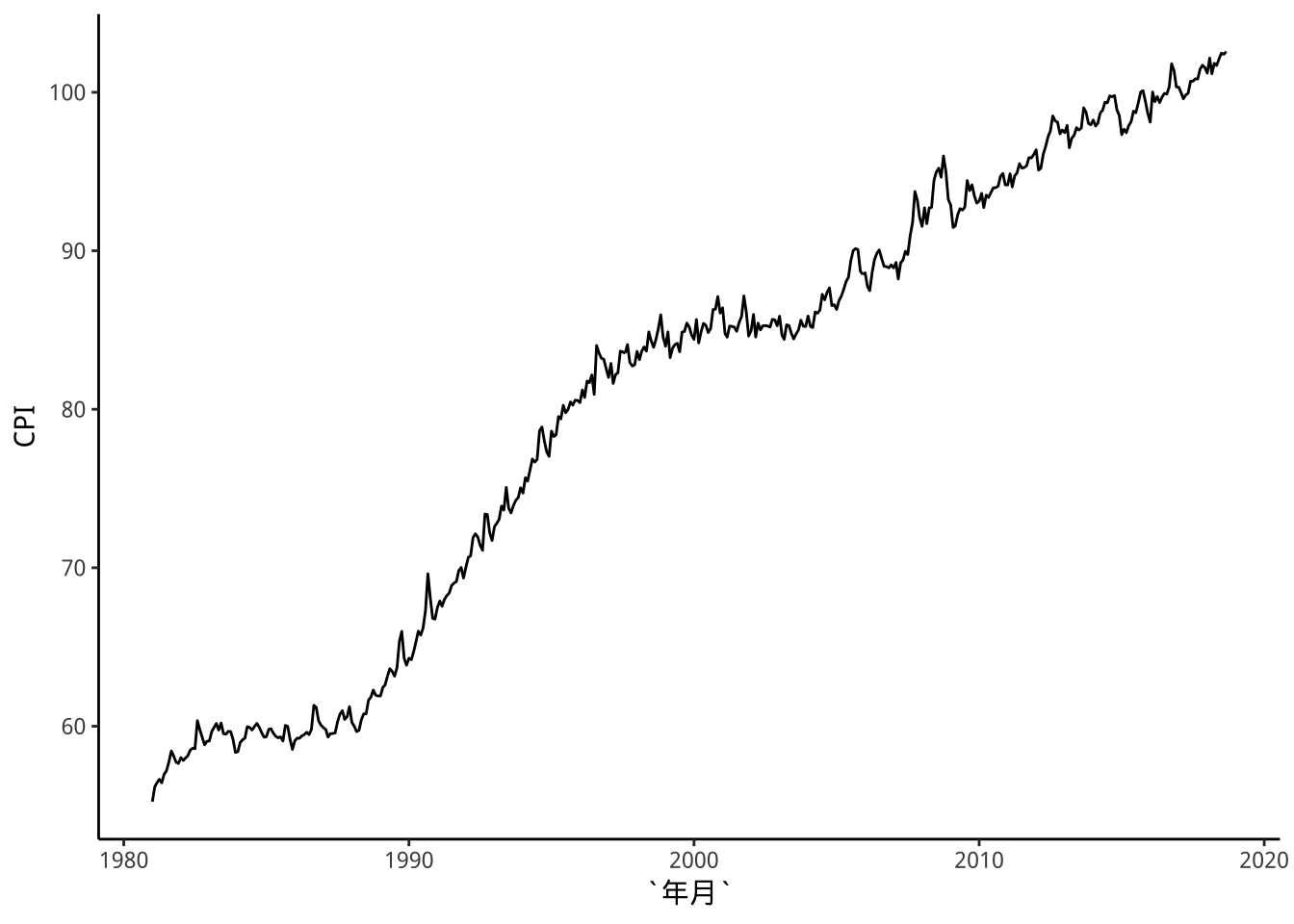

5.5.1 limits: 上下限

NA：表示沒設限

basePlot+
  scale_x_date(limits=c(ymd("2003-01-01"),NA))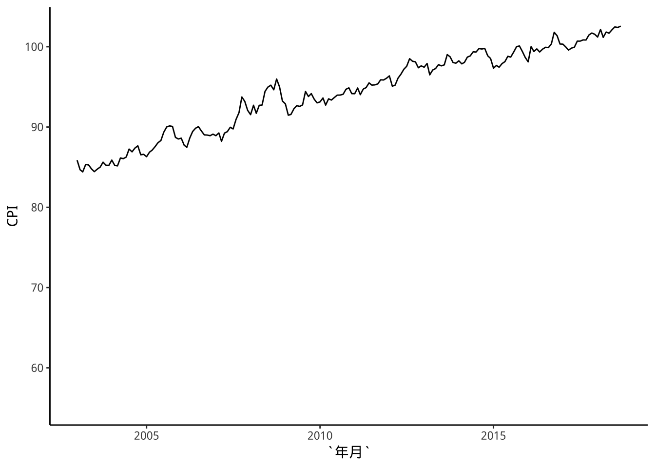

適用於任何scale

basePlot+
  scale_x_date(limits=c(ymd("2003-01-01"),NA))+
  scale_y_continuous(limits=c(80,NA))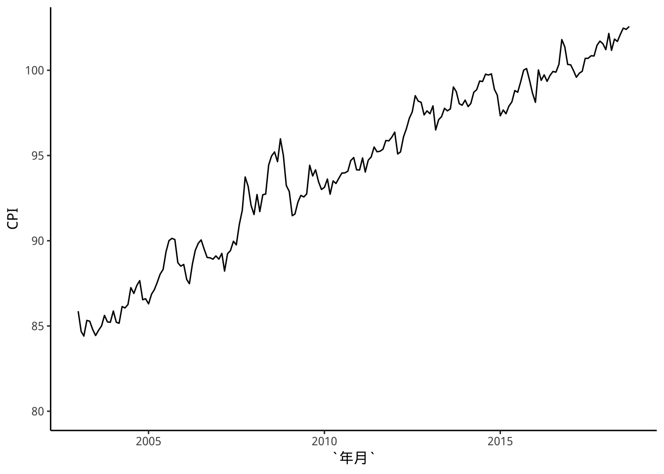

改成2003M1為基期,其指數為100

dataCPI %>% filter(年月==ymd("2003-01-01")) %>% 
  select(CPI) -> CPI2003M1
dataCPI %>% 
  mutate(CPI=CPI/CPI2003M1$CPI*100) -> dataCPI2

新基期圖形

dataCPI2 %>% ggplot()+
  geom_line(aes(x=年月,y=CPI)) -> basePlot2
basePlot2

5.5.2 breaks: 軸標標示點

標示點英文為tick

未設標示點

basePlot2內含y下限

basePlot2 +
  scale_y_continuous(limits=c(95,NA)) -> basePlot2
basePlot2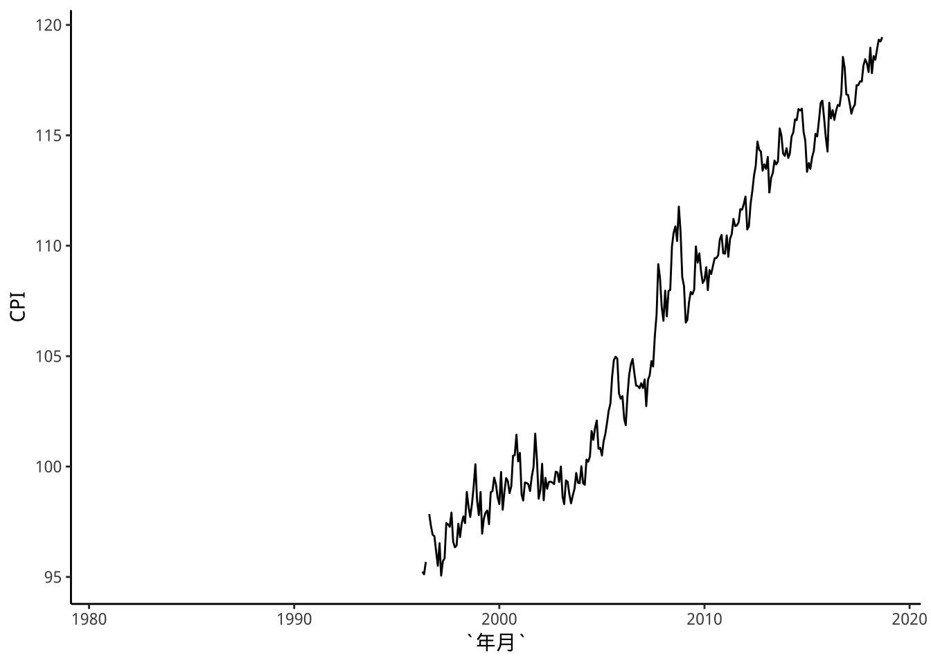

basePlot2增加x下限

basePlot2 +
  scale_x_date(limits=c(ymd("2003-01-01"),NA))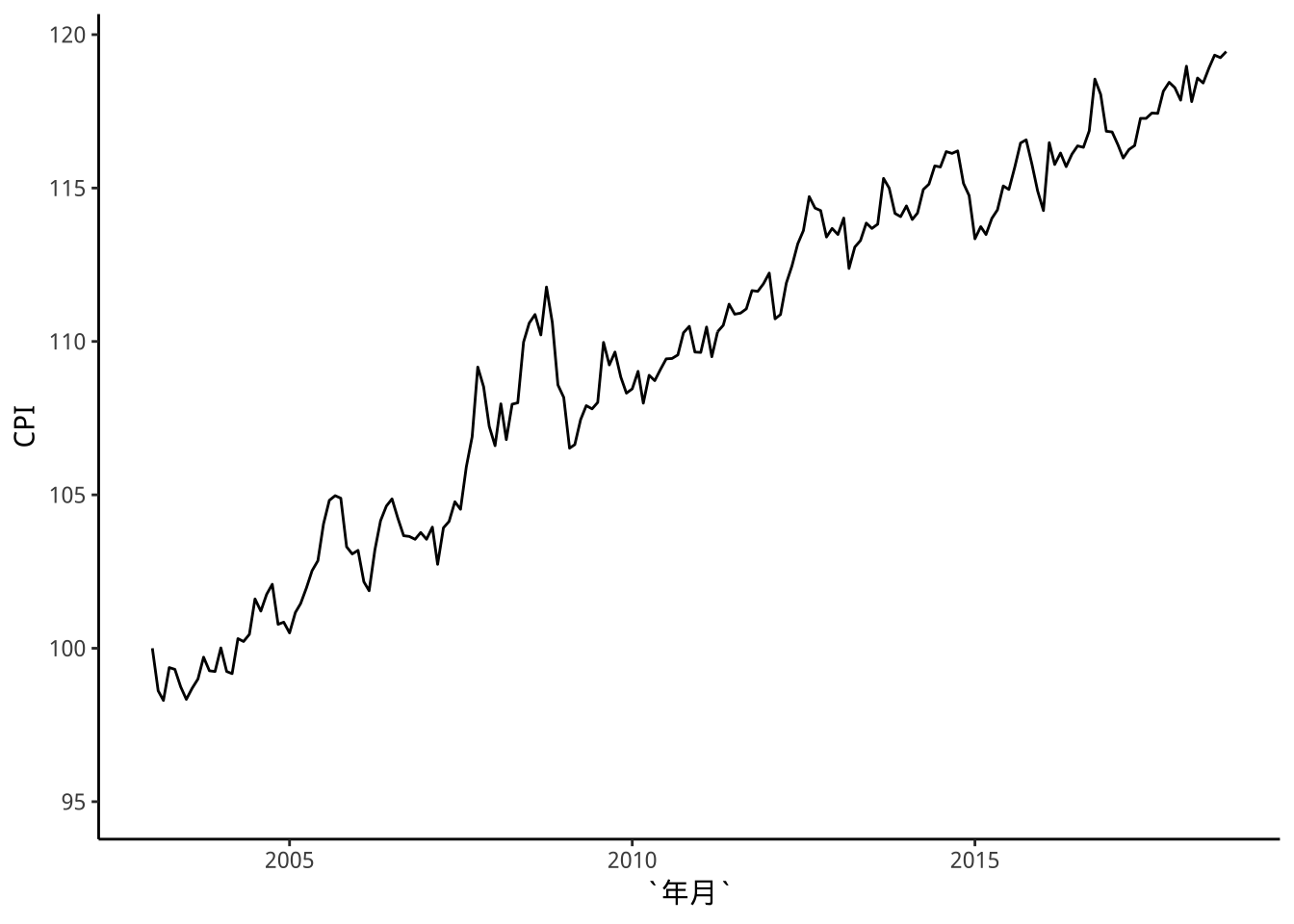

5.5.2.1 有設標示點

breakDates <- c("2003-01-01",
                "2005-01-01","2010-01-01","2015-01-01",
                "2018-01-01")
breakDates %>% ymd() -> breakDates
basePlot2 +
  scale_x_date(limits=c(ymd("2003-01-01"),NA),
               breaks = breakDates)

5.5.3 labels: 軸標標示點名稱

手動設標示點名稱

breakDates <- c("2003-01-01",
                "2005-01-01","2010-01-01","2015-01-01",
                "2018-01-01")
breakDates %>% ymd() -> breakDates

breakLabels <- c("2003",
                 "2005","2010","2015",
                 "2018")
basePlot2 +
  scale_x_date(limits=c(ymd("2003-01-01"),NA),
               breaks = breakDates,
               labels = breakLabels)

函數設標示點名稱

函數必需能由breaks input產生字串output

basePlot2 +
  scale_x_date(limits=c(ymd("2003-01-01"),NA),
               breaks = breakDates,
               labels = function(x) year(x))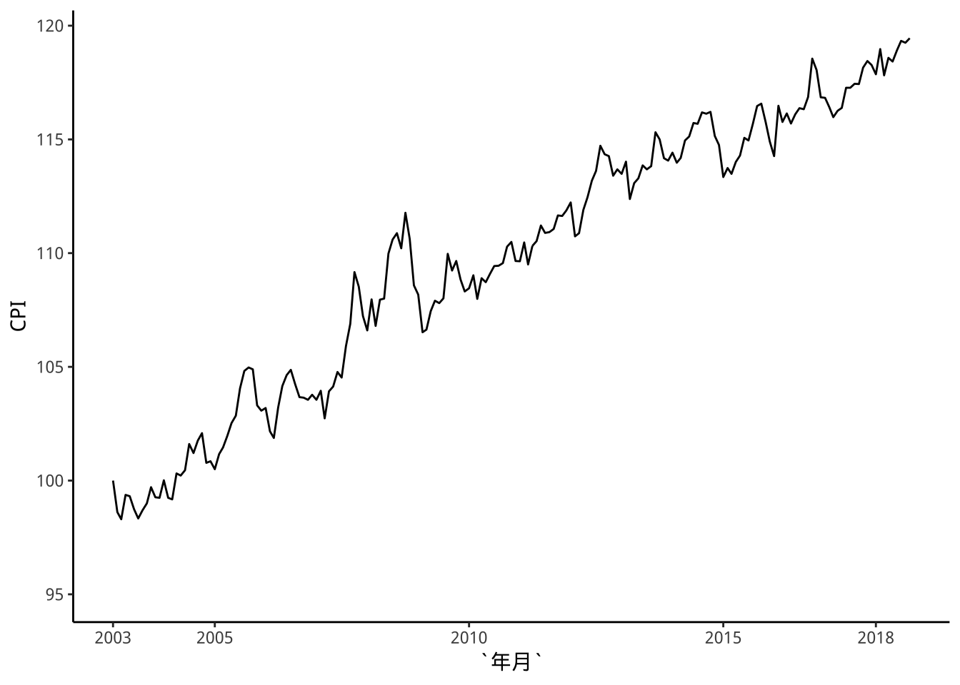

請將年月標示名稱改成民國年表示。