5.1 Voronoi tesselation
Voronoi tessellation uses seeds to calculate Voronoi regions. For every seed there is one Voronoi region that contains the area that is closest to the particular seed. There are two seed specifications we are interested in:
Tower locations as seeds –> n = n = 1746
Coverage area centroid (per antenna) locations as seeds –> n = 5191
We will focus on both specifications in parallel.
As mentioned above Voronoi regions contains the area that is closest to the particular seed, in our case the position of each tower represents a seed and each tile is allocated to its closest seed. This means that the Voronoi specification only relies on the distance between tile and tower. However, as we will see later on, there are tiles that need to be split up because the exact distance calculations do not use the centroid of a tile as reference but the whole area. Therefore, certain tiles need to be split up according to their area into different Voronoi regions. This will be further explained later on.
Furthermore, when using Voronoi tesselation with towers as seeds we need to further prepare our c.vector object as it is currently structured on the antenna level. For this we need to aggregate it on to the tower level, meaning a tower is associated with as many phones its respective antenna is associated with. We then join the Voronoi regions with the tiles to create an object that links tiles within respective Voronoi regions.
For any kind of Voronoi tessellation we need to work with the grid level data (tiles) and the cell coverage data (tower, antennas).
# aggregating the antennas to towers (and corresponding values) and identifying problematic tower locations (outside of focus area)
tower.aggr <- coverage.areas.comp %>%
  st_drop_geometry() %>%
  group_by(tower.ID) %>%
  mutate(phones.sum = sum(phones.sum)) %>%
  distinct(tower.ID, .keep_all = T) %>%
  ungroup() %>%
  dplyr::select(tower.ID, X.tow, Y.tow, phones.sum) %>%
  st_as_sf(coords = c("X.tow", "Y.tow")) %>%
  st_sf(crs = 3035) %>%
  mutate(within.fa = lengths(st_within(., census.geo.body))) # find seeds outside the focus area

# saving towerIDs of problematic towers
towers.outside.ID <- tower.aggr %>%
  filter(within.fa == 0) %>%
  dplyr::select(tower.ID) %>%
  deframe()

# filtering unproblematic towers
towers.inside <- tower.aggr %>%
  filter(within.fa == 1)

# Finding respective nearest point on focus area border for every problematic tower location and binding the unproblematic towers back
# this object contains the final seed locations in the geometry
towers.final.data <- tower.aggr %>%
  filter(within.fa == 0) %>%
  st_nearest_points(., census.geo.body) %>%
  st_cast("POINT") %>%
  .[seq(2, length(.), 2)] %>% #
  st_as_sf() %>%
  mutate(tower.ID = towers.outside.ID) %>%
  mutate(geometry = x) %>%
  st_sf(sf_column_name = "geometry") %>%
  dplyr::select(-x) %>%
  bind_rows(towers.inside)

sum(unlist(st_intersects(towers.final.data, census.geo.body))) == length(tower.aggr$tower.ID) # check if all are within now
## [1] TRUE# Using the seed object to calculate the Voronoi regions
tower.seed.voronoi <- towers.final.data %>%
st_geometry() %>%
st_union() %>%
st_voronoi() %>%
st_collection_extract(type = "POLYGON") %>%
st_sf(crs = 3035) %>%
st_join(tower.aggr) %>% # rejoin with seed object to retain seed id
st_intersection(census.geo.body) %>%
mutate(category.log = log10(phones.sum / as.numeric(st_area(geometry)))) %>%
mutate(category = cut(category.log, c(-6, -4, -2, -1), right = F, ordered_result = T))## Warning: attribute variables are assumed to be spatially constant throughout all
## geometriesAnd now the same preparation for the coverage area centroids (here also just “antennas” even though this is imprecise). When using antennas as seed points, we can use the original structure of the c.vector and define the Voronoi regions.
### antennas
# aggregating the antennas to towers (and corresponding values) and identifying problematic tower locations (outside of focus area)
antenna.aggr <- coverage.areas.comp %>%
  st_drop_geometry() %>%
  dplyr::select(antenna.ID, geometry = antenna.centroid, phones.sum) %>%
  st_sf() %>%
  st_sf(crs = 3035) %>%
  mutate(within.fa = lengths(st_within(., census.geo.body))) # find seeds outside the focus area

# saving towerIDs of problematic antennas
antennas.outside.ID <- antenna.aggr %>%
  filter(within.fa == 0) %>%
  dplyr::select(antenna.ID) %>%
  deframe()

# filtering unproblematic antennas
antennas.inside <- antenna.aggr %>%
  filter(within.fa == 1)

# Finding respective nearest point on focus area border for every problematic antenna location and binding the unproblematic towers back
# this object contains the final seed locations in the geometry
antennas.final.data <- antenna.aggr %>%
  filter(within.fa == 0) %>%
  st_nearest_points(., census.geo.body) %>%
  st_cast("POINT") %>%
  .[seq(2, length(.), 2)] %>% #
  st_as_sf() %>%
  mutate(antenna.ID = names(antennas.outside.ID)) %>%
  mutate(geometry = x) %>%
  st_sf(sf_column_name = "geometry") %>%
  dplyr::select(-x) %>%
  bind_rows(antennas.inside)

sum(unlist(st_intersects(antennas.final.data, census.geo.body))) == length(antenna.aggr$antenna.ID) # check if all are within now
## [1] TRUE# Using the seed object to calculate the Voronoi regions
antenna.seed.voronoi <- antennas.final.data %>%
st_geometry() %>%
st_union() %>%
st_voronoi() %>%
st_collection_extract(type = "POLYGON") %>%
st_sf(crs = 3035) %>%
st_join(antenna.aggr) %>% # rejoin with seed object to retain seed id
st_intersection(census.geo.body) %>%
mutate(category.log = log10(phones.sum / as.numeric(st_area(geometry)))) %>%
mutate(category = cut(category.log, c(-6, -4, -2, -1), right = F, ordered_result = T))## Warning: attribute variables are assumed to be spatially constant throughout all
## geometries# check density values
# antenna.seed.voronoi %>%
# ggplot() +
# geom_density(aes(category.log))
# Visualizing the Vornoi regions with respective phone count
VT.plot <- tower.seed.voronoi %>%
ggplot() +
geom_sf(aes(fill = category), size = 0.001) +
scale_fill_ptol(na.translate = FALSE) +
scale_color_ptol(na.translate = FALSE) +
guides(color = F) +
labs(fill = "Local density\n(log10)") +
ggtitle("Voronoi tower", subtitle = "Tower locations as seeds") +
theme(axis.text.x = element_text(angle = 90, hjust = 1))
saveRDS(VT.plot, "C:/Users/Marco/Vysoká škola ekonomická v Praze/Tony Wei Tse Hung - YAY/working objects/VT.plot.rds")
VA.plot <- antenna.seed.voronoi %>%
ggplot() +
geom_sf(aes(fill = category), size = 0.001) +
scale_fill_ptol(na.translate = FALSE) +
scale_color_ptol(na.translate = FALSE) +
guides(color = F) +
labs(fill = "Local density\n(log10)") +
ggtitle("Voronoi antenna", subtitle = "Coverage area centroid locations as seeds") +
theme(axis.text.x = element_text(angle = 90, hjust = 1))
saveRDS(VA.plot, "C:/Users/Marco/Vysoká škola ekonomická v Praze/Tony Wei Tse Hung - YAY/working objects/VA.plot.rds")
VT.plot
VA.plot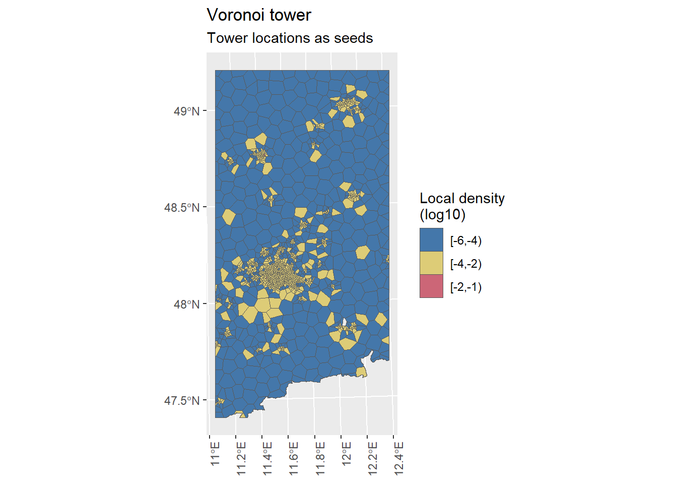

Figure 5.1: The tower centroids were used as seeds for the creation of the Voronoi regions.
We have now created the Voronoi regions for our focus area with tower locations as seeds as well as with antenna respective coverage area centroid locations as seeds. The number of seeds and Voronoi regions align with each other.
The spatial density per tile can be expressed as the ratio of the mobile phones in that region and the area of the Voronoi region:
\(d_{k} = \frac{\sum c_{i}} {A_{k}}\)
This region specific estimand corresponds to the tile estimate for a tile that is contained in this region. On the tile level there can be two cases that we need to differentiate:
Tiles that are completely contained within one Voronoi region
Tiles that intersect with two or more Voronoi regions
For the first case, the tile specific estimate corresponds to \(d_{k}\). For the second case we will calculate a weighted mean of the relevant Voronoi region estimates by using the corresponding tile area within each Voronoi region as weights.
# spatial densities per Voronoi region
tower.voronoi.est <- tower.seed.voronoi %>%
  mutate(area = as.numeric(st_area(.$geometry))) %>%
  mutate(voronoi.est = phones.sum / area) # the sum of the product of this and the area is the total pop


# Joining the regions with the tile specific data
tower.seed.voronoi.join <- tower.voronoi.est %>%
  st_join(census.de.100m.tile.pop) %>% # & re-connect the data items
  st_set_agr("aggregate") %>% # clean up
  group_by(internal.id) %>%
  mutate(count = n()) %>%
  ungroup()

# identifiying tiles intersecting with multiple Voronoi regions
tower.multiple <- tower.seed.voronoi.join %>%
  st_drop_geometry() %>%
  filter(count > 1) %>%
  distinct(internal.id) %>%
  deframe()

# calculate area within competing voronoi regions of "multiple" tiles
tower.intersect.tiles <- census.de.100m.tile.pop %>%
  filter(internal.id %in% tower.multiple) %>%
  st_intersection(tower.voronoi.est) %>%
  st_collection_extract(type = "POLYGON") %>% # select the polygons
  mutate(amount.tiles = as.numeric(st_area(.$geometry)) / 10000) # checked if it adds up to 1
## Warning: attribute variables are assumed to be spatially constant throughout all
## geometries## Warning in st_collection_extract.sf(., type = "POLYGON"): x is already of type
## POLYGON.The second case can be visualized as follows:
example.helper <- tower.intersect.tiles %>%
  filter(internal.id == "254331") %>%
  dplyr::select(tower.ID) %>%
  deframe()

# bird example plot
VT.bird.example.plot <- tower.intersect.tiles %>%
  filter(internal.id == "254331") %>%
  ggplot() +
  geom_sf(color = "black") +
  geom_sf(data = (census.de.100m.tile.pop %>% filter(internal.id == "254331")), color = "red", fill = NA) +
  geom_sf(data = (tower.seed.voronoi %>% filter(tower.ID %in% example.helper)), fill = NA) +
  labs("Birds view of a tile that intersects with
multiple regions", x = "", y = "") +
  theme(axis.text.x = element_text(angle = 90, hjust = 1))

# saveRDS(VT.bird.example.plot, "C:/Users/Marco/Vysoká škola ekonomická v Praze/Tony Wei Tse Hung - YAY/working objects/VT.bird.example.plot.rds")

VT.example.plot <- tower.intersect.tiles %>%
  filter(internal.id == "254331") %>%
  ggplot() +
  geom_sf() + # add description and scales
  geom_sf_label(aes(label = tower.ID)) +
  geom_sf_text(aes(label = paste0("(", round(amount.tiles, 2), ")")), nudge_y = -7) +
  geom_sf(data = (census.de.100m.tile.pop %>%
  filter(internal.id == "254331")), color = "red", fill = NA) +
  labs(title = "Relative area per Voronoi region", x = "", y = "") +
  theme(axis.text.x = element_text(angle = 90, hjust = 1))

# saveRDS(VT.example.plot, "C:/Users/Marco/Vysoká škola ekonomická v Praze/Tony Wei Tse Hung - YAY/working objects/VT.example.plot.rds")

VT.bird.example.plot
VT.example.plot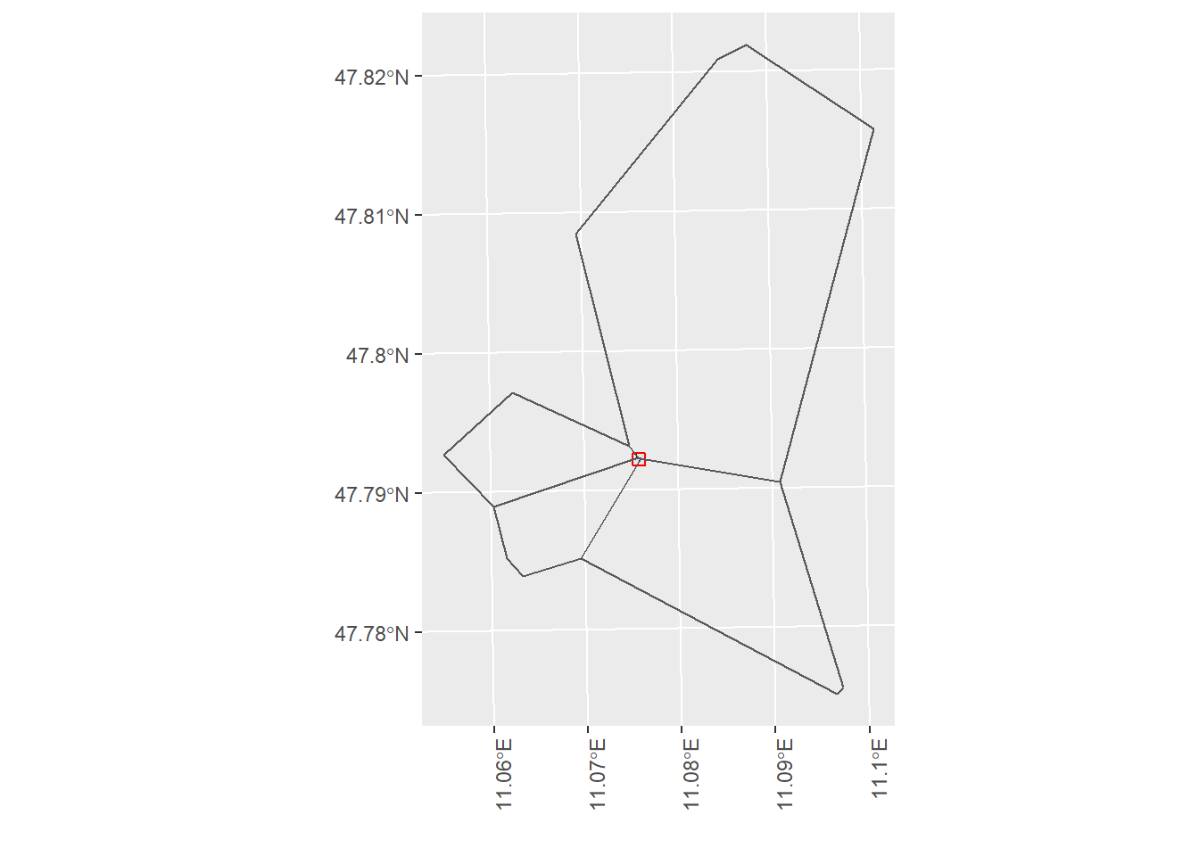
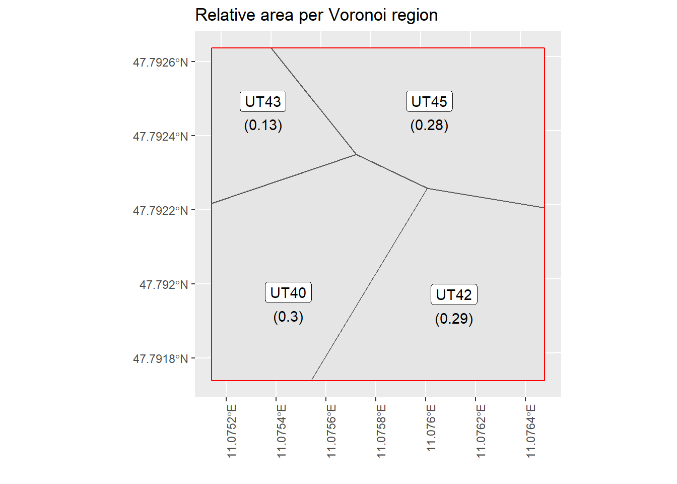
Figure 5.2: This is an example of a tile that intersects with multiple Voronoi regions. The labels and number correspond to the Voronoi region and the given area that are used as weights for the weighted mean estimator.
Here we visualize the second case with an example tile and the respective Voronoi regions from the Voronoi tower specification. In the left plot we can see a small tile that is indicated in red. This tile is at the intersection of 4 Voronoi regions. The corresponding relative tile area intersecting with each Voronoi region can be seen in the right plot. The labels correspond to the Voronoi region ID and the values below in brackets indicate the proportional weight that should be considered in calculting the tile specific weighted mean estimate. To compare this to the first case - where a tile is fully contained only in one region - the weight for the particular Voronoi region is 1. The same methodogolgy is pursued for the Voronoi antenna case.
And now the same again for the antennas.
# spatial densities per Voronoi region
antenna.voronoi.est <- antenna.seed.voronoi %>%
  mutate(area = as.numeric(st_area(.$geometry))) %>%
  mutate(voronoi.est = phones.sum / area) # the sum of the product of this and the area is the total pop


# Joining the regions with the tile specific data
antenna.seed.voronoi.join <- antenna.voronoi.est %>%
  st_join(census.de.100m.tile.pop) %>% # & re-connect the data items
  st_set_agr("aggregate") %>% # clean up
  group_by(internal.id) %>%
  mutate(count = n()) %>%
  ungroup()

# identifiying tiles intersecting with multiple Voronoi regions
antenna.multiple <- antenna.seed.voronoi.join %>%
  st_drop_geometry() %>%
  filter(count > 1) %>%
  distinct(internal.id) %>%
  deframe()

# calculate area within competing voronoi regions of "multiple" tiles
antenna.intersect.tiles <- census.de.100m.tile.pop %>%
  filter(internal.id %in% antenna.multiple) %>%
  st_intersection(antenna.voronoi.est) %>%
  st_collection_extract(type = "POLYGON") %>% # select the polygons
  mutate(amount.tiles = as.numeric(st_area(.$geometry)) / 10000) # checked if it adds up to 1
## Warning: attribute variables are assumed to be spatially constant throughout all
## geometriesWe can now calculate the estimated spatial density per tile. For furter understanding: Each tile that is completely contained within one Voronoi region will have the identical tile specific estimate as the remaining tiles that are completely contained within the same Voronoi region. Each tile that is contained in multiple Voronoi region will be a weighted estimate from the Voronoi region tile estimates according to their area specific weight.
#### Towers

# final datatset to calculate spatial density
tower.voronoi.final <- tower.intersect.tiles %>%
  st_drop_geometry() %>%
  dplyr::select(internal.id, tower.ID, amount.tiles) %>%
  right_join(tower.seed.voronoi.join, by = c("internal.id", "tower.ID")) %>%
  mutate(amount.tiles = case_when(is.na(amount.tiles) ~ 1,
                                  TRUE ~ amount.tiles)) %>%
  group_by(internal.id) %>%
  mutate(voronoi.est.tower = weighted.mean(x = voronoi.est, w = amount.tiles) * 10000) %>%
  ungroup() %>%
  distinct(internal.id, voronoi.est.tower) # should result in same length as the raw tiles object and the sum of the vornoir est corrected should resemble the sum of the c.vec

#### antennas

# final datatset to calculate spatial density
antenna.voronoi.final <- antenna.intersect.tiles %>%
  st_drop_geometry() %>%
  dplyr::select(internal.id, antenna.ID, amount.tiles) %>%
  right_join(antenna.seed.voronoi.join, by = c("internal.id", "antenna.ID")) %>%
  mutate(amount.tiles = case_when(is.na(amount.tiles) ~ 1,
                                  TRUE ~ amount.tiles)) %>%
  group_by(internal.id) %>%
  mutate(voronoi.est.corrected = weighted.mean(x = voronoi.est, w = amount.tiles) * 10000) %>%
  ungroup() %>%
  distinct(internal.id, voronoi.est.corrected, pop) # should result in same length as the raw tiles object and the sum of the vornoir est corrected should resemble the sum of the c.vec

voronoi.final.both <- antenna.voronoi.final %>%
  mutate(voronoi.est.antenna = voronoi.est.corrected) %>%
  dplyr::select(-voronoi.est.corrected) %>%
  left_join(tower.voronoi.final, by = "internal.id") %>%
  mutate(voronoi.est.antenna = voronoi.est.antenna + 3 / n()) # adjusting size due to rounding error

# saveRDS(voronoi.final.both, "C:/Users/Marco/Vysoká škola ekonomická v Praze/Tony Wei Tse Hung - YAY/Estimates/Voronoi both/Voronoi.estimates.rds")
We have now created a results object, voronoi.final.both that is structured on the tile level with the variables internal.id (tile specific ID), pop (true mobile phone population per tile), voronoi.est.antenna (the tile specific Voronoi estimate with the antenna specification) and voronoi.est.tower (the tile specific Voronoi estimate with the tower specification). The tile specific estimates can therefore be directly compared to the true tile specific population. This performance control will be executed later on in the chapter Evaluation. The next subchapter will describe the other estimation approach, MLE Poisson.