4.2 Generation of Mobile Phone Population
Our toy world bases on population census data from the German Federal Statistical Office [2] (https://www.destatis.de/EN/Home/_node.html). This data entails continuous population counts on a 100m * 100m geographical grid.
# Raw census 100 m^2 data read in
census.raw <- fread("C:/Users/Marco/Vysoká škola ekonomická v Praze/Tony Wei Tse Hung - YAY/Data/Census data Germany/csv_Bevoelkerung_100m_Gitter/Zensus_Bevoelkerung_100m-Gitter.csv")

census.raw %>%
  dplyr::select(x = x_mp_100m, y = y_mp_100m, pop.raw = Einwohner) %>%
  sample_n(10) %>%
  datatable()
census.raw contains 4 columns, the tile ID, the x and y coordinate of the tiles left bottom corner and the number of inhabitants associated with the tile. For statistical disclosure reasons tiles containing less than 3 inhabitants have perturbed values. The value -1 stands for a tile with less than 3 inhabitants. The specific perturbation is explained further in the explanatory notes of the raw data.
For computational reasons, the following analysis will only focus on a subset of the tiles located in the state of Bavaria, which is situated in the south-east of Germany. We chose this area because it comprises a high diversity of urban, suburban, and rural areas, enabling us to focus on the parameter of population density. This zone is identified by a longitude between 4400000 and 4500000 and a latitude between 2700000 and 2900000.
# Bounding box of focus area
bb.focus.dat <- data.frame(xmin = 4400000, xmax = 4500000,
                           ymin = 2700000, ymax = 2900000)
bb.focus.vec <- c(xmin = 4400000, xmax = 4500000,
                  ymin = 2700000, ymax = 2900000)

# Download data from : https://gadm.org/download_country_v3.html --> R(sf) level 1
# This data is only used for visualization purposes and not further needed for the rest of the analysis
germany.raw <- readRDS("C:/Users/Marco/Vysoká škola ekonomická v Praze/Tony Wei Tse Hung - YAY/working objects/gadm36_DEU_1_sf.rds")

germany <- germany.raw %>%
  st_transform(crs = 3035)

focus.area.plot <- germany %>%
  ggplot() +
  geom_sf() +
  geom_rect(data = bb.focus.dat, aes(ymin = ymin, ymax = ymax,
                                      xmin = xmin, xmax = xmax,
                                     color = "red"),
            size = 1, fill = "transparent") +
  ggtitle(label = "Focus area of analysis") +
  scale_color_identity(name = "",
                       labels = c("Focus area"),
                       guide = "legend") +
  labs(x = NULL, y = NULL) +
  theme(axis.text.x = element_text(angle = 90, hjust = 1))

saveRDS(focus.area.plot, "C:/Users/Marco/Vysoká škola ekonomická v Praze/Tony Wei Tse Hung - YAY/Plots/focus.area.rds")

focus.area.plot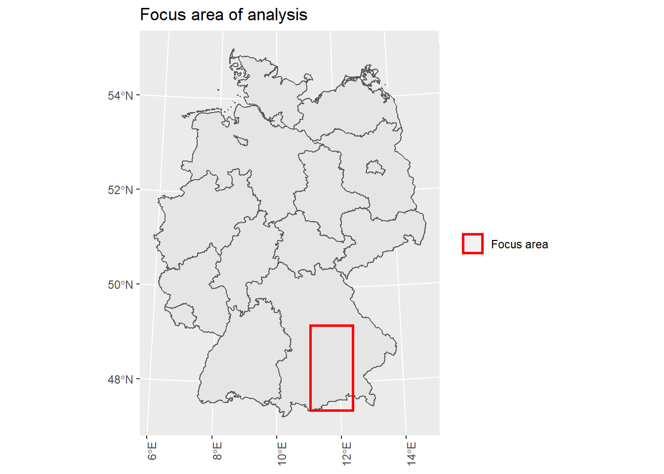
Figure 4.1: For computational reasons we will only focus on a subset of the tiles located in the state of Bavaria because it comprises high diversity in urban, suburban, and rural areas
We will therefore exclude the tiles that are not contained in this bounding box. Next, we need to define valid values for population values in tiles that contain undisclosed values. We create the variable pop.pert and sample from the values 0 and 1 equally if the value in pop.raw is -1, we sample from the values 2 and 3 equally if the value is 2 or 3, and we copy the values for pop.pert from pop.raw if they are larger than 3. This follows the logic of the perturbation methods mentioned above. For our final population variable, pop, which will also represent our ground truth population, we aim to reach a total value of about a third of the perturbed population, pop.pert. The reason for this reduction is the use case of working with data from one MNO provider. We assume this MNO provider covers about 1/3 of all inhabitants’ phones. Therefore, our measurement unit in the following concerns mobile phones.
For the creation of pop we split the tiles according to pop.pert into 2 groups:
1. tiles below or equal to 40,
2. tiles above 40.
census <- census.raw %>%
  dplyr::select(x = x_mp_100m, y = y_mp_100m, pop.raw = Einwohner) %>%
  filter(between(y, 2700000, 2900000), #
         between(x, 4400000, 4500000)) %>%
  mutate(internal.id = row_number()) %>%  # create new ID variable
  mutate(pop.pert = case_when(pop.raw == "-1" | is.na(pop.raw) ~ sample(0:1, n(), replace = T),
                              pop.raw %in% c(2:3) ~ sample(2:3, n(), replace = T),
                              TRUE ~ as.integer(pop.raw)))

census %>%
  mutate(pop.group = case_when(pop.pert <= 40 ~ "Less or equal 40",
                               pop.raw > 40 ~ "More than 40")) %>%
  group_by(pop.group) %>%
  summarise(n.tiles = n()) %>%
  datatable()
## `summarise()` ungrouping output (override with `.groups` argument)For the first group we will sample from a Binomial distribution with N as the number of phones per tile, pop.pert and a success probability of 1/3. For the second group we will copy the value from pop.pert and divide it by 3.
# Dataframe with bounding box, tile id, and two versions of the population variable
census.pop.new <- census %>%
  mutate(bin.helper = case_when(pop.pert <= 40 ~ sample(0:1, n(), prob = c(2/3, 1/3), replace = T),
                                pop.pert > 40 ~  NA_integer_)) %>%
  mutate(pop = case_when(bin.helper == 1 ~ pop.pert,
                         bin.helper == 0 ~ as.integer(0),
                         is.na(bin.helper) ~ as.integer(round(pop.pert / 3, 0))))

sum(census.pop.new$pop.pert)
## [1] 5353914sum(census.pop.new$pop) # should yield about 1/3 of pop.pert## [1] 1786344This operationalization yields about 1/3 of pop.pert.
As mentioned above, this area is very heterogeneous in urban-rural intensity. Knowing the location of urban centers is very important for the corresponding radio cell network as there are differences in cell coverage between these different area kinds. We are aiming at developing a 3-category classification for each tile: Rural, Suburban and Urban. Based on the census data we cannot locate urban centers just yet. Classifying tiles on such a low spatial resolution into one of these categories independent from each other (i.e. based on their population numbers) would not lead to the true location of urban centers; in fact, we need to take spatial dependence into consideration in order to identify urban centers. Therefore we apply a spatial clustering algorithm to account for the spatial dependence.
In order to run the clustering algorithm, we again form two groups according to pop:
1. tiles below 15,
2. tiles above or equal 15.
census.cluster <- census.pop.new %>%
  mutate(pop.raster = case_when(pop < 15 ~ 1,
                                pop >= 15 ~ 2)) %>%
  dplyr::select(-pop.raw)

# saveRDS(census.cluster, "C:/Users/Marco/Vysoká škola ekonomická v Praze/Tony Wei Tse Hung - YAY/working objects/example data frame.rds")
census.cluster <- readRDS("C:/Users/Marco/Vysoká škola ekonomická v Praze/Tony Wei Tse Hung - YAY/working objects/example data frame.rds")

census.cluster %>%
  group_by(pop.raster) %>%
  summarise(n.tiles = n()) %>%
  datatable()
## `summarise()` ungrouping output (override with `.groups` argument)The group formation is saved in pop.raster. We will only use the second group for the clustering. These tiles represent so to say seed points for the occurrence of agglomerations.
For clustering we will use the cca() function from the osc package. The input data needs to be a raster object, therefore we will transform census.cluster data frame into a raster brick. We will set our coordinate reference system (depends on the input data, here “3035”). The final input object for the cca() function is the raster layer that contains the pop.raster dummy variable.
# Raster brick object of the complete bounding box region
census.tile <- raster::rasterFromXYZ(census.cluster, crs = st_crs(3035)$proj4string)
## Warning in showSRID(uprojargs, format = "PROJ", multiline = "NO"): Discarded
## datum Unknown based on GRS80 ellipsoid in CRS definition## Warning in matrix(values, nrow = ncell(x), ncol = nlayers(x)): Datenlänge
## [9999184] ist kein Teiler oder Vielfaches der Anzahl der Zeilen [2000000]# Raster layer object with specified dichotomized variable for cca
census.tile.pop.raster <- raster::raster(census.tile,
layer = 5) # this needs to be the index of the pop.raster variable
set.seed(20)
# CCA workflow, clustering 1 values (pop > 15)
cities <- cca(census.tile.pop.raster,
cell.class = 2, # indicating that only tiles with "1" in pop should be used for clustering
s = 11100000, # radius/shell size of burning clustering procedure
unit = "m") ## [1] "get coordinates:"
##
|
| | 0%
|
|================== | 25%
|
|=================================== | 50%
|
|==================================================== | 75%
|
|======================================================================| 100%
## [1] "use as X-coordinates column ' x '"
## [1] "use as Y-coordinates column ' y '"
## [1] "Sorting... Done"
## [1] "Start Clustering..."
## [1] "Clustering... Done"
## [1] "Summary... Done"# number of unique clusters
length(cities$size)## [1] 16444This leads to 16444 unique clusters of varying sizes. This is still a very large number and we aim to reduce it. We can now assign a cluster.id to each of the tiles in group 2 back in our originalcensus.cluster data frame. In order to receive a sf object, which is advantageous for spatial data analysis, we need to rasterize the cluster results. We do this per cluster and use a paralized workflow to decrease computation time. Furthermore, we classify clusters into two groups:
1. Clusters, with less than 10 tiles,
2. Cluster with more or equal to 10 tiles.
# Adding classification results to census.cluster sf object and splitting it up for further parallelized workflow
census.classified.sf <- cities[["cluster"]] %>%
  right_join(census.cluster, by = c("long" = "x", "lat" = "y")) %>%
  mutate(parts = ntile(internal.id, 50)) %>%
  group_by(parts) %>%
  group_split()

# Calculate the number of cores
no_cores <- availableCores() - 1
plan(multisession, workers = no_cores)

# Rasterizing the sf object with cluster results and transforming back to final sf object
census.classified.sf.transform <- census.classified.sf %>%
  future_map(~raster::rasterFromXYZ(., crs = st_crs(3035)$proj4string), .progress = T) %>%
  future_map(~st_as_stars(.), .progress = T) %>%
  future_map_dfr(~st_as_sf(., coords = c("long", "lat")), .progress = T) %>%
  st_transform(crs = 3035) %>%
  group_by(cluster_id) %>%
  mutate(cluster.tile.n = n()) %>%
  ungroup() %>%
  dplyr::select(-parts) %>%
  mutate(pop.area.kind.helper = case_when(pop.raster != 0 & cluster.tile.n > 10 ~ 1, # specify clusters that have at least 10 tiles
                                          TRUE ~ 0))

census.classified.sf.transform %>%
  st_drop_geometry() %>%
  ungroup() %>%
  filter(pop.area.kind.helper == 1) %>%
  summarise(n.cluster.unique = n_distinct(cluster_id)) %>%
  as_vector()
## n.cluster.unique
## 276By differentiating by cluster size, we can exclude the small clusters and therefore reduce the number of unique clusters to the more sensible number of 276. These represent the largest spatial agglomerations of tiles that contain more than 15 people.
# summarise clusters geometries to build buffers
result.interim <- census.classified.sf.transform %>%
  filter(pop.area.kind.helper == 1 & !is.na(cluster_id)) %>%
  group_by(cluster_id) %>%
  summarise(geometry = st_union(geometry))
## `summarise()` ungrouping output (override with `.groups` argument)# build buffers for suburban and urban area respectively
urban.buffer <- st_buffer(result.interim, 800)
suburban.buffer <- st_buffer(result.interim, 3000)
# classify tiles that are within the respective buffer with either suburban or urban, rest is rural
census.classified.final.sf <- census.classified.sf.transform %>%
mutate(urban.dummy = lengths(st_within(census.classified.sf.transform, urban.buffer))) %>%
mutate(suburban.dummy = lengths(st_within(census.classified.sf.transform, suburban.buffer))) %>%
mutate(pop.area.kind = case_when(urban.dummy > 0 ~ "Urban",
suburban.dummy > 0 & urban.dummy == 0 ~ "Suburban",
TRUE ~ "Rural"))
# saveRDS(census.classified.final.sf, file = "C:/Users/Marco/Vysoká škola ekonomická v Praze/Tony Wei Tse Hung - YAY/working objects/census.classified.final.sf.rds")
# census.classified.final.sf <- readRDS("C:/Users/Marco/Vysoká škola ekonomická v Praze/Tony Wei Tse Hung - YAY/working objects/census.classified.final.sf.rds")
## derive the shape of the focus area
# census.geo.body <- census.de.100m.tile %>%
# select(internal.id) %>%
# summarise(geometry = st_union(geometry))
# saveRDS(census.geo.body, "Vysoká škola ekonomická v Praze/Tony Wei Tse Hung - YAY/working objects/shape.focusarea.rds")
census.geo.body <- readRDS("C:/Users/Marco/Vysoká škola ekonomická v Praze/Tony Wei Tse Hung - YAY/working objects/shape.focusarea.rds")
# check if correctly classified
cluster.plot2 <- census.classified.final.sf %>%
filter(pop.area.kind %in% c("Suburban", "Urban")) %>%
ggplot() +
geom_sf(aes(color = factor(pop.area.kind), fill = factor(pop.area.kind)), show.legend = F) +
scale_color_manual(breaks = c("Suburban", "Urban"), values = c("#DDCC77", "#CC6677")) +
labs(x = "", y = "", title = "Clustering results", size = 20) +
theme(axis.text.x = element_text(angle = 90, hjust = 1))
# saveRDS(cluster.plot2, "C:/Users/Marco/Vysoká škola ekonomická v Praze/Tony Wei Tse Hung - YAY/working objects/cluster.plot2.rds")Tiles that are within the colored boundaries are classified either as Suburban or Urban. The outer tiles are classified as Rural.
census.classified.final.sf %>%
  st_drop_geometry() %>%
  group_by(pop.area.kind) %>%
  summarise(n.tiles = n(), n.tiles.prop = round(n() / length(census.classified.final.sf$pop.area.kind), 2)) %>%
  datatable()
## `summarise()` ungrouping output (override with `.groups` argument)Suburban or Urban. To better understand the relationship between number of mobile phones and the classified area we can visualize this distribution with an Empirical Cumulative Distribution Function (ECDF) and the complement of it, the Empirical Complementary Cumulative Distribution Function (ECCDF).
## This function computes ECCDF data frames with log10 transformations of the x and y axis

custom_ecdf_prep <- function(df) {
  data <- df %>%
    mutate(pop.plot = pop + 1) %>%
    arrange(pop.plot) %>%
    mutate(prob = 1 / n()) %>%
    mutate(cum.prob = cumsum(prob)) %>%
    mutate(cum.prob.comp = 1 - cum.prob) %>%
    mutate(log10.cum.prob.comp = log10(cum.prob.comp)) %>%
    mutate(log10.pop = log10(pop.plot)) %>%
    mutate(cum.prob.comp = 1 - cum.prob)

  return(data)
}


pop.true.ECCDF <- census.classified.final.sf %>%
  st_drop_geometry() %>%
  ungroup() %>%
  custom_ecdf_prep() %>%
  dplyr::select(log10.cum.prob.comp, log10.pop, pop.area.kind) %>%
  mutate(log10.cum.prob.comp = round(log10.cum.prob.comp, 3)) %>% # effective plot sample --> faster plotting excluding overplot
  distinct()
## Warning in mask$eval_all_mutate(dots[[i]]): NaNs wurden erzeugtpop.true.ECDF <- census.classified.final.sf %>%
st_drop_geometry() %>%
ungroup() %>%
custom_ecdf_prep() %>%
dplyr::select(cum.prob.comp, pop.plot, pop.area.kind) %>%
mutate(cum.prob.comp = round(cum.prob.comp, 3)) %>% # effective plot sample --> faster plotting excluding overplot
distinct()## Warning in mask$eval_all_mutate(dots[[i]]): NaNs wurden erzeugtbreaks.first <- c("Rural", "Suburban", "Urban")
ECCDF.pop.plot <- pop.true.ECCDF %>%
ggplot() +
geom_point(aes(x = log10.pop, y = log10.cum.prob.comp,
color = pop.area.kind)) +
geom_hline(yintercept = -0.3010300, linetype = "dotted") +
geom_hline(yintercept = -1, linetype = "dotted") +
geom_text(x = 1.5, y = -0.15, label = "50% of the data") +
geom_text(x = 1.5, y = -0.8, label = "90% of the data") +
scale_color_ptol(breaks = breaks.first) +
ggtitle("Mobile phone density per tile") +
labs(y = "log10(Prob(Y > x))", x = "log10(Mobile phones)",
colour = "") +
ylim(-7, 0) +
theme(legend.position = "bottom")
ECDF.pop.plot <- pop.true.ECDF %>%
ggplot() +
geom_point(aes(x = pop.plot, y = cum.prob.comp, color = pop.area.kind)) +
scale_color_ptol(breaks = breaks.first,
guide = FALSE, expand = c(0, 0)) +
xlim(0, 30) +
labs(y = "", x = "") +
theme(plot.title = element_text(size = 10, face = "bold", hjust = 0.5),
plot.subtitle = element_text(size = 9, hjust = 0.5),
axis.title.x = element_blank(),
axis.title.y = element_blank())
pop.dist.ecdf.insert.plot <- ECCDF.pop.plot +
annotation_custom(ggplotGrob(ECDF.pop.plot),
xmin = 0, xmax = 1.5,
ymin = -7, ymax = -3)## Warning: Removed 310 rows containing missing values (geom_point).# saveRDS(pop.dist.ecdf.insert.plot, "C:/Users/Marco/Vysoká škola ekonomická v Praze/Tony Wei Tse Hung - YAY/Plots/pop.dist.ecdf.insert.plot.rds")# Geographical distribution of the true population
true.pop.data <- census.classified.final.sf %>%
mutate(pop.cat = case_when(pop <= 1 ~ "Less or equal 1",
pop > 1 & pop <= 10 ~ "Between 2 and 10",
pop > 10 & pop <= 30 ~ "Between 11 and 30",
pop > 30 ~ "More than 30")) %>%
mutate(mobile = factor(pop.cat, levels = c("Less or equal 1", "Between 2 and 10", "Between 11 and 30", "More than 30"))) %>%
group_by(mobile) %>%
summarise(geometry = st_union(geometry))
# saveRDS(true.pop.data, "C:/Users/Marco/Vysoká škola ekonomická v Praze/Tony Wei Tse Hung - YAY/Estimates/Plot.files/true.pop.data.rds")
true.pop.geo.plot <- true.pop.data %>%
ggplot() +
geom_sf(aes(fill = mobile, color = mobile)) +
scale_fill_ptol(name = "# Mobile phones") +
scale_color_ptol(guide = F) +
labs(x = "", y = "", title = "True population value in size categories") +
theme(axis.text.x = element_text(angle = 90, hjust = 1))
# saveRDS(true.pop.geo.plot, "C:/Users/Marco/Vysoká škola ekonomická v Praze/Tony Wei Tse Hung - YAY/Estimates/Plot.files/true.pop.geo.plot.rds")pop.dist.ecdf.insert.plot## Warning: Removed 1 rows containing missing values (geom_point).true.pop.geo.plot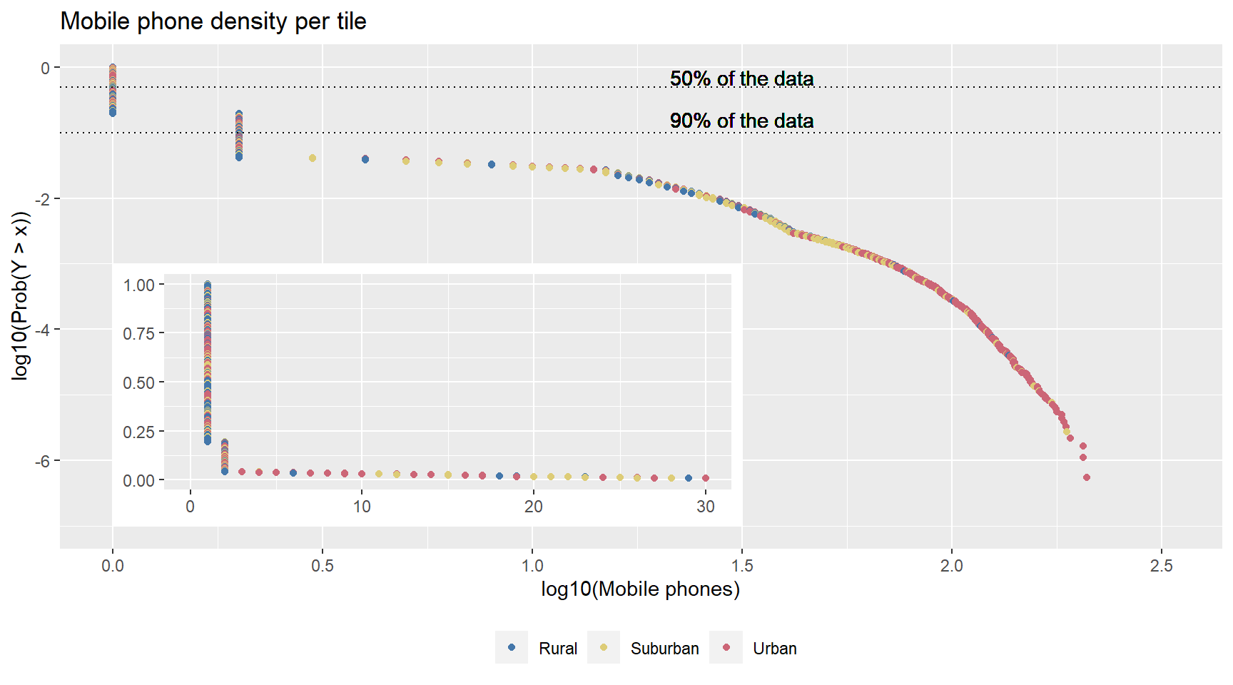
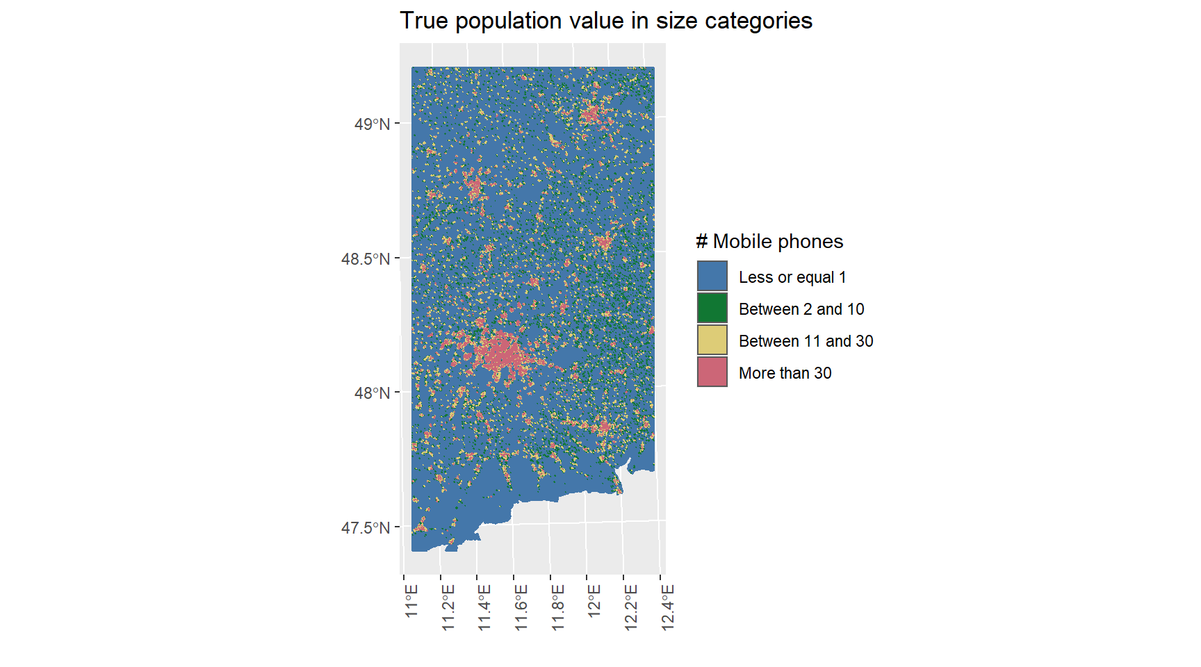
Figure 4.2: …
The ECCDF is a step function and it is commonly used with variables that have a highly skewed distribution. We can see that this is the case - the population on this low spatial resolution is heavily right skewed. We can also notice that our spatial clustering approach worked because even though most high populated tiles are most often classified as Urban, there are some Urban and Suburban tiles with low number of mobile phones. For more complete plotting we added 1 to pop because otherwise tiles with 0 mobile phones would not be visualized due to the log transformation.
The tile classification marks an important interim result in the Generation of our Toy World. We now have an interesting mobile phone population situated in a area-diverse geography, being able to differentiate between Rural, Suburban and Urban areas. In the next part we will use the area classification, pop.area.kind, as a basis for the generation of a synthetic Radio Network.