4.4 Device to cell association
For this subchapter we need to load the following packages.
library(tidyverse)
library(data.table)
library(sf)
library(furrr)
library(Matrix)
##
## Attaching package: 'Matrix'## The following objects are masked from 'package:tidyr':
##
## expand, pack, unpacklibrary(ggthemes)The fact that we allow for overlapping coverage areas means that mobile phones have different antennas they can connect to, when being at a location that is multiply covered. In our toy world this makes it possible to associate mobile phones to antennas in a stochastic manner. This is also the reason why we cannot know yet, how many phones are assigned to each antenna. With overlapping coverage areas, we let a relevant subset of antennas compete for the mobile phones which are in their reach. This will be dependent on the signal strength parameter.
This part will establish the association between mobile phones of a generic tile to a relevant antenna. The result will be a reference matrix \(P\) of size \(I x J\), where \(I\) denotes the total number of radio cells (antennas), \(J\) is the total number of tiles, and the elements correspond to the probability of the mobile phones of any tile \(j\) which are registered in the cell \(i\). With \(P\) one is able to simulate a column vector \(c\) (random variable) which describes the total count of mobile phones associated to a radio cell.
We assume that \(\mathcal{L}_{j}\) denotes the subset of radio cells covering a particular tile. This means that these respective radio cells are competing with each other to be associated with the cell phones in the tile. We therefore assign probabilities which describe the respective association between a radio cell \(i\) and tile \(j\).
For this probability we first determine the signal strength which we model with a received signal strength indication. This function computes the signal a mobile phone receives from any relevant antenna, mostly dependent on the distance between the transmitter (antenna) and receiver (mobile phone) and the terrain. Signal propagation is therefore modelled as
\[ S_{ij} = S_{0} - S_{dist}(d_{ij}), \] where \(d_{ij}\) describes the distance between the \(i\)’th antenna coverage area centroid and the \(j\)’th tile centroid in meter distance, \(S_{0}\) is the signal strength at \(d_{0} = 1\) meter distance from the antenna in decibel milliwatt (dBm). \(S_{0}\) describes the power \(P\) of the antenna in Watt at the location of the antenna. This can be transformed into dBm:
\[ S_{0} = 30 + 10 log_{10}(P). \] \(S_{dist}(d)\) describes the loss of the signal strength as a function of \(d\):
\[ S_{dist}(d) = 10 \gamma log_{10}(d) \] Here, \(\gamma\) describes the path loss exponent, which will differ depending on the kind of terrain the coverage area is located in. In our case we will approximate this with the type of layer the antenna is labeled with.
In other words, the received signal \(S_{ij}\) is the difference between the maximum signal strength (being at the closest point to the antenna) and the total signal loss depending on the distance between the antenna and the tile, and the terrain.
signal_strength_rec <- Vectorize(function(power.wt, distance.m, loss.exp, max.equal = -60) {

  power.db <- 30 + 10 * log10(power.wt)
  path.loss.db <- 10 * loss.exp * log10(distance.m)
  rec.signal.db <- power.db - path.loss.db

  if (rec.signal.db > max.equal) { # maximum sij where it doesnt make a difference anymore if closer
    rec.signal.db.adjusted <- max.equal
  } else {
    rec.signal.db.adjusted <- rec.signal.db
  }

  return(rec.signal.db.adjusted)
})


signal_dominance <- Vectorize(function(layer, rec.signal.db.adjusted, min.threshold = -110,
                                       s.mid = c(-65, -70, -100, -45), s.steep = c(0.2, 0.2, 0.3, 0.2)) {

  if (rec.signal.db.adjusted < min.threshold) {
    signal.dom <- 0
  } else if (layer == "Rural") {
    signal.dom <- 1 /  (1 + exp(-s.steep[1] * (rec.signal.db.adjusted - s.mid[1])))
  } else if (layer == "Suburban") {
    signal.dom <- 1 /  (1 + exp(-s.steep[2] * (rec.signal.db.adjusted - s.mid[2])))
  } else if (layer == "Urban") {
    signal.dom <- 1 /  (1 + exp(-s.steep[3] * (rec.signal.db.adjusted - s.mid[3])))
  } else {
    signal.dom <- 1 /  (1 + exp(-s.steep[4] * (rec.signal.db.adjusted - s.mid[4])))
  }

  return(signal.dom)
})

sim <- tibble(id = 1:27000,
              dist.sij.m = c(1:12000, 1:2500, 1:500, 1:12000),
              loss.exp = c(rep(3.85, 12000), rep(4.5, 2500), rep(5.5, 500), rep(3.85, 12000)),
              power.wt = c(rep(20, 12000), rep(10, 2500), rep(5, 500), rep(20, 12000)),
              area.kind = c(rep("Rural", 12000), rep("Suburban", 2500), rep("Urban", 500), rep("Extreme", 12000))) %>%
  mutate(signal.sij.rec = signal_strength_rec(power.wt = power.wt,
                                              distance.m = dist.sij.m,
                                              loss.exp = loss.exp)) %>%
  mutate(signal.sij.dom = signal_dominance(layer = area.kind, rec.signal.db.adjusted = signal.sij.rec))
  # mutate(signal.strength.cat = factor(case_when(signal.sij.rec >= (-70) ~ "Excellent",
  #                                        signal.sij.rec < (-70) & signal.sij.rec >= (-90) ~ "Good",
  #                                        signal.sij.rec < (-90) & signal.sij.rec >= (-100) ~ "Fair",
  #                                        signal.sij.rec < (-100) & signal.sij.rec >= (-110) ~ "Poor",
  #                                        signal.sij.rec < (-110) ~ "No signal")))


signal.strength.plot <- sim %>%
  ggplot() +
  geom_point(aes(x = dist.sij.m, y = signal.sij.rec, color = area.kind)) +
  scale_color_ptol(breaks = c("Extreme", "Rural", "Suburban", "Urban"),
                   labels = c("Extreme", "Rural", "Suburban", "Urban")) +
  labs(title = "Received signal strength based on distance and antenna layer",
       subtitle = "Simulated data for relevant antenna radii",
       x = "Distance between antenna coverage area centroid and tile centroid in m",
       y = "Received signal strength in dBm",
       color = "Layer")
# saveRDS(signal.strength.plot, "C:/Users/Marco/Vysoká škola ekonomická v Praze/Tony Wei Tse Hung - YAY/working objects/signal.strength.plot.rds")

signal.strength.plot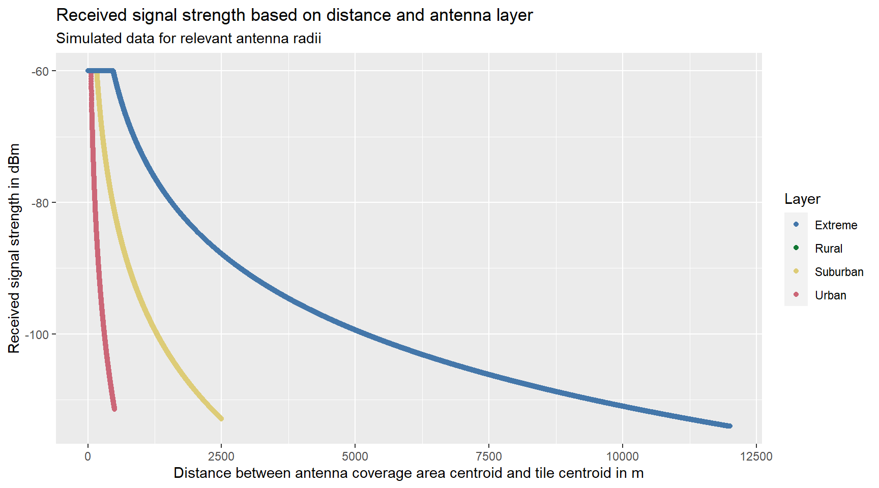
Figure 4.7: …
Power \(P\) and loss exponent \(\gamma\) are layer specific - we assume higher power for antennas with greater coverage areas and higher loss exponents for greater noise potential such as urban areas. For layer 1 antennas we specify Power value \(P\) of 20W and a loss exponent \(\gamma\) of 3.85, for layer 2 10W and 4.5 and for layer 3 5W and 5.5, respectively.
In the figure above we can see that antennas with greater power and smaller loss exponent (e.g. layer 1) transmits stronger signal for greater distances. \(S_{ij}\) values higher than -60 are capped at -60 because a better signal strength should not increase the probability of a mobile phone to be connected to this particular antenna. The range of received signal strength lies between -60 (“Excellent”) to <-110 (“No signal”).
However, \(S_{ij}\) is scaled in dBm, for our device to cell association we need a likelihood which is scaled between 0 and 1. Therefore, we use the concept of signal dominance introduced in … This concept entails the idea of load balancing, trying to avoid monster antennas, i.e. there is a certain limiting capacity of mobile phones each antenna can carry. Furthermore, signal dominance, \(S_{strength}(ij)\) is expressed and scaled as the connection likelihood. We use a logistic function defined as:
\[ S_{strength}(ij) = \frac{1}{1 + exp(-0.2 (S_{ij} - (-92.5))} \]
Here, -92.5 describes the midpoint and 0.2 the steepness of the curve, both scaled in dBm. These values can of course be adjusted based on the specific load balancing assumptions. We can visualize this function for our simulated dataset:
signal.dominance.plot <- sim %>%
  ggplot() +
  geom_point(aes(x = signal.sij.rec, y = signal.sij.dom, color = area.kind)) +
  geom_vline(xintercept = -110, linetype = "dotted") +
  annotate(geom = "text", x = -112, y = 0.4,
           label = "Min. threshold at -110dBm", linetype = "dotted",
           angle = 90) +
  scale_color_ptol(breaks = c("Extreme", "Rural", "Suburban", "Urban"),
                   labels = c("Extreme", "Rural", "Suburban", "Urban")) +
  labs(title = "Logistic relation between received signal strength and signal dominance",
       x = "Received signal strength in dBm", y = "Signal dominance",
       color = "Signal strength cat.")
## Warning: Ignoring unknown parameters: linetypesaveRDS(signal.dominance.plot, "C:/Users/Marco/Vysoká škola ekonomická v Praze/Tony Wei Tse Hung - YAY/working objects/signal.dominance.plot.rds")
signal.dominance.plot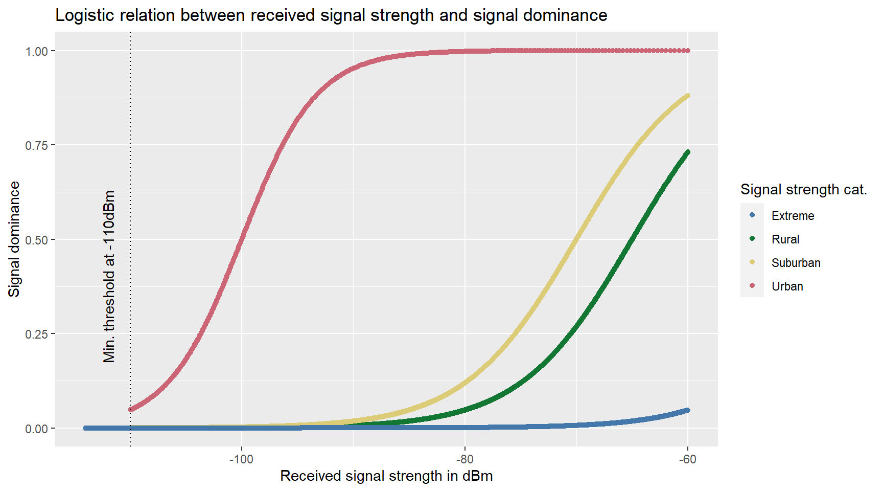
Figure 4.8: …
Finally, we can use this connection likelihood, \(S_{strength}(ij)\), to model overlapping antenna competition. The elements of \(P\) - the probability with which the mobile phones within a particular cell are associated with a particular radio cell - are defined by
\[ p_{ij} = \frac{S_{strength}(ij)}{\sum_{i \in \mathcal{L}_{j}} S_{strength}(ij)} \]
where \(S_{strength}(ij)\) describes the signal dominance of a particular antenna \(i\) associated with a particular tile \(j\), and \(\mathcal{L}_{j}\) describes the subset of radio antennas that are covering the tile \(j\). We then simulate the tile specific experiments - every mobile phone within a tile will be independently assigned to relevant radio cell with the probability \(p_{ij}\).
Currently, we have exemplified the device-to-cell-association with a small simulated dataset. We will focus now on the implementation of this process within our toyworld. As a first step we need to spatially join the radio network, coverage.areas.final with our population, census.classified.final.sf and calculate the distance between any tile centroid and any antenna, dist.sij.
dev.to.cell.join <- census.classified.final.sf %>%
  mutate(tile.centroid = st_centroid(geometry)) %>%
  st_join(coverage.areas.final, left = F) %>%
  st_transform(crs = 3035) %>%
  st_sf(sf_column_name = "antenna.centroid", crs = 3035) %>%
  mutate(dist.sij = as.numeric(st_distance(tile.centroid, antenna.centroid, by_element = T)))

# saveRDS(dev.to.cell.join, "C:/Users/Marco/Vysoká škola ekonomická v Praze/Tony Wei Tse Hung - YAY/working objects/dev.to.cell.join.adj.rds")
Then we calculate the received signal strength, signal.sij.rec, the signal dominance, signal.sij.dom and finally the rescaled version, namely \(p_{ij}\), which will call weight.pij.
# run in loop to discard extreme antennas
dev.to.cell.metric <- dev.to.cell.join %>%
  st_drop_geometry() %>%
  select(internal.id, antenna.ID, pop, area.kind, dist.sij) %>%
  mutate(power.wt = case_when(area.kind == "Rural" ~ 20,
                              area.kind == "Suburban" ~ 10,
                              area.kind == "Urban" ~ 5),
         loss.exp = case_when(area.kind == "Rural" ~ 3.85,
                              area.kind == "Suburban" ~ 4.5,
                              area.kind == "Urban" ~ 5.5)) %>%
  mutate(signal.sij.rec = signal_strength_rec(power.wt = power.wt, distance.m = dist.sij,
                                              loss.exp = loss.exp)) %>%
  mutate(signal.sij.dom = signal_dominance(layer = area.kind,
                                           rec.signal.db.adjusted = signal.sij.rec)) %>%
  # mutate(signal.strength.cat = factor(case_when(signal.sij.rec >= (-70) ~ "Excellent",
  #                                        signal.sij.rec < (-70) & signal.sij.rec >= (-90) ~ "Good",
  #                                        signal.sij.rec < (-90) & signal.sij.rec >= (-100) ~ "Fair",
  #                                        signal.sij.rec < (-100) & signal.sij.rec >= (-110) ~ "Poor",
  #                                        signal.sij.rec < (-110) ~ "No signal"))) %>%
  group_by(internal.id) %>%
  mutate(weight.pij = case_when(is.nan(as.numeric(signal.sij.dom / sum(signal.sij.dom, na.rm = T))) ~ as.numeric(0),
                                TRUE ~ as.numeric(signal.sij.dom / sum(signal.sij.dom, na.rm = T)))) %>%
  ungroup() %>%
  mutate(mp.est = weight.pij * pop)


# run in loop
sum.mp.per.antenna <- dev.to.cell.metric %>%
  group_by(antenna.ID) %>%
  summarise(mp.est.sum = sum(mp.est), wgt.avg.weight = weighted.mean(weight.pij, mp.est)) %>%
  mutate(extreme = case_when(mp.est.sum > 3000 ~ 1,
                             TRUE ~ 0)) %>%
  select(antenna.ID, extreme)

dev.to.cell.metric.new <- dev.to.cell.metric %>%
  left_join(sum.mp.per.antenna, by = "antenna.ID") %>%
  mutate(area.kind = case_when(extreme == 1 ~ "Extreme",
                               TRUE ~ area.kind)) %>%
  select(internal.id, antenna.ID, pop, area.kind, dist.sij, signal.sij.rec) %>%
  mutate(signal.sij.dom = signal_dominance(layer = area.kind,
                                           rec.signal.db.adjusted = signal.sij.rec)) %>%
  group_by(internal.id) %>%
  mutate(weight.pij = case_when(is.nan(as.numeric(signal.sij.dom / sum(signal.sij.dom, na.rm = T))) ~ as.numeric(0),
                                TRUE ~ as.numeric(signal.sij.dom / sum(signal.sij.dom, na.rm = T)))) %>%
  ungroup() %>%
  mutate(mp.est = weight.pij * pop)

sum.mp.per.antenna.adj <- dev.to.cell.metric.new %>%
  # st_drop_geometry() %>%
  group_by(antenna.ID) %>%
  summarise(mp.est.sum = sum(mp.est), wgt.avg.weight = weighted.mean(weight.pij, mp.est))


# saveRDS(dev.to.cell.metric.new, "C:/Users/Marco/Vysoká škola ekonomická v Praze/Tony Wei Tse Hung - YAY/working objects/dev.to.cell.metric.adjusted.final.rds")
dev.to.cell.metric is basically a long format version of \(P\). After calculating weight.pij we can differentiate all tile into 4 categories:
* Tiles with no mobile phones
* Tiles covered completely by only one antenna
* Tiles covered by multiple antennas
* Tiles with mobile phones and not sufficiently covered by at least one antenna
dev.to.cell.classified <- dev.to.cell.metric.new %>%
  dplyr::select(internal.id, antenna.ID, pop, weight.pij) %>%
  mutate(coverage.kind = case_when(pop == 0 ~ "0 population",
                                   pop >= 1 & weight.pij == 1 ~ "covered completely by one antenna",
                                   pop >= 1 & weight.pij > 0 & weight.pij < 1 ~ "covered by multiple antennas",
                                   pop >= 1 & weight.pij == 0 ~ "tile covered unsufficiently"))

# saveRDS(dev.to.cell.classified, "C:/Users/Marco/Vysoká škola ekonomická v Praze/Tony Wei Tse Hung - YAY/working objects/dev.to.cell.classified.final.rds")
# dev.to.cell.classified <- readRDS("C:/Users/Marco/Vysoká škola ekonomická v Praze/Tony Wei Tse Hung - YAY/working objects/dev.to.cell.classified.final.rds")

# aggregating and specifing the tiles that are uncovered
tiles.cat <- dev.to.cell.classified %>%
  # st_drop_geometry() %>%
  filter(!weight.pij == 0) %>%
  dplyr::select(internal.id, coverage.kind) %>%
  group_by(internal.id) %>%
  summarise(count = n())
## `summarise()` ungrouping output (override with `.groups` argument)# how many tiles are not sufficiently covered
missings <- anti_join(census.classified.final.sf, tiles.cat, by = "internal.id")
length(missings$internal.id)## [1] 0This classification will speed the further process as we only need to run the stochastic process of assigning mobile phones to antennas for the tiles that are covered by multiple antennas. Mobile phones within tiles that are completely covered only by one antenna can be assigned as a whole to the relevant antenna. A special case are tiles that are not covered sufficiently, i.e. they have no non-zero weight.pij value. We build this category to check if this characteristic applies. If a tile is not covered and has no mobile phone population then this aspect can be ignored.
coverage.intensity <- tiles.cat %>%
  left_join(census.classified.final.sf, by = "internal.id") %>%
  dplyr::select(internal.id, count, pop.area.kind) %>%
  arrange(count) %>%
  mutate(prob = 1 / n()) %>%
  mutate(cum.prob = cumsum(prob))


coverage.intensity.plot <- coverage.intensity %>% # tiles.cat
  ggplot() +
  stat_count(aes(count), fill = "#4477A9") +
  geom_vline(xintercept = mean(coverage.intensity$count), linetype = "solid", color = "#117733", size = 1.5) +
  geom_vline(xintercept = median(coverage.intensity$count), linetype = "solid", color = "#CC6677", size = 1.5) +
  annotate("text", x = median(coverage.intensity$count) + 2, y = 5e+05, color = "#CC6677",
           label = paste("Median =", median(coverage.intensity$count))) +
  annotate("text", x = round(mean(coverage.intensity$count), 2) - 3, y = 5e+05, color = "#117733",
           label = paste("Mean =", round(mean(coverage.intensity$count), 2))) +
  labs(y = "Count of tiles", x = "Covered by ... antennas", colour = "",
       title = "Number of antennas covering a tile")
coverage.intensity.plot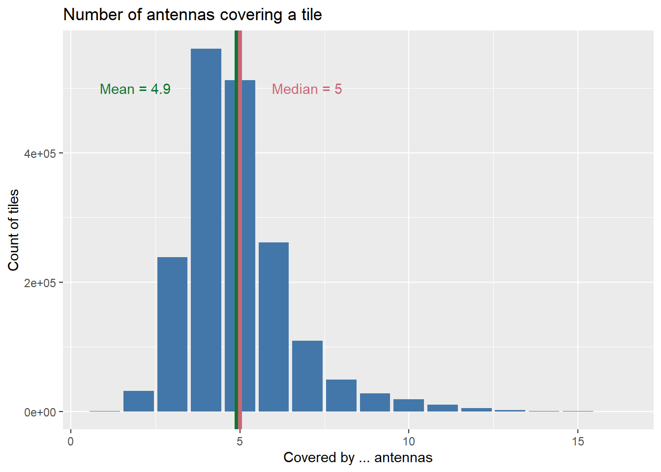
Figure 4.9: The distribution is right skewed with a mean of 4.9, a minimum of 1, and a maximum of 16 antenna(s) per tile.
The figure above shows a histogram representing the number of antennas per tile. The distribution is right skewed with a mean of 4.9, a minimum of 1 and a maximum of 16 antenna(s) per tile. So, we have a median of 5 antennas per tile, which is a more robust measure than the mean that is driven by the extreme values. Even though the coverage areas were generated synthetically, this distribution mimics a realistic layout.
The next step is to start with the construction of the column vector \(c\). All phones from tiles that are completely covered by only antenna can be put into the object C.vec.fixed.helper.
# Differentiating workflows between device to cell associations depending on coverage.kind variable
# One object where tiles are completely covered by one cell (no stochastic process)
C.vec.fixed.helper <- dev.to.cell.classified %>%
  filter(coverage.kind == "covered completely by one antenna") %>%
  dplyr::select(antenna.ID, pop)
# saveRDS(C.vec.fixed.helper, "C:/Users/Marco/Vysoká škola ekonomická v Praze/Tony Wei Tse Hung - YAY/working objects/C.vec.fixed.helper.rds")
Then we construct an object that contains all tile-antenna connections and split it into a large list according to the internal.id. Each element of the list will therefore contain all tile-antenna association of a respective tile. We can then run the stochastic assignment process within each list element, C.vec.multiple. To increase speed we can run this is parallel, because each assignment process is independent. For assignment we sample the each phone of a tile to the relevant antennas with sampling weights, weight.pij.
# One object where tiles are covered by multiple cells
C.vec.multiple.helper <- dev.to.cell.classified %>%
  filter(coverage.kind == "covered by multiple antennas") %>%
  group_split(internal.id)

# Dropping associations for tiles with 0 population and tiles which are not sufficiently covered (in this case the coverage network was optimized that every tile is sufficiently covered)

# saveRDS(C.vec.multiple.helper, "C:/Users/Marco/Vysoká škola ekonomická v Praze/Tony Wei Tse Hung - YAY/working objects/C.vec.multiple.helper.rds")
# C.vec.multiple.helper <- readRDS("Vysoká škola ekonomická v Praze/Tony Wei Tse Hung - YAY/working objects/C.vec.multiple.helper.rds")

# Calculate the number of cores
no_cores <- availableCores() - 1
plan(multisession, workers = no_cores)

set.seed(5)

C.vec.multiple <- C.vec.multiple.helper %>%
  future_map(~sample(x = .$antenna.ID, mean(.$pop),
                     replace = T, prob = .$weight.pij), .progress = T) %>%
  future_map(as_tibble, .id = "internal.id", .progress = T) %>%
  future_map(~group_by(., value), .progress = T) %>%
  future_map(~summarise(., pop.count.rand = n(), .groups = "drop"), .progress = T)

# saveRDS(C.vec.multiple, "C:/Users/Marco/Vysoká škola ekonomická v Praze/Tony Wei Tse Hung - YAY/working objects/C.vec.multiple.rds")

C.vec.df <- C.vec.multiple %>%
  bind_rows() %>%
  dplyr::select(antenna.ID = value, pop = pop.count.rand) %>%
  bind_rows(C.vec.fixed.helper) %>%
  group_by(antenna.ID) %>%
  summarise(phones.sum = sum(pop))

# saveRDS(C.vec.df, "C:/Users/Marco/Vysoká škola ekonomická v Praze/Tony Wei Tse Hung - YAY/working objects/C.vec.df.final.new.rds")
Then, we can append both objects (C.vec.fixed.helper and C.vec.multiple) together sum all mobile phones by antenna. The result is the column vector \(c\) which will act as a reference (ground truth) for the later on introduced estimation strategies.
!!!
# ECCDF of population distribution
ECCDF.phones.data <- C.vec.df %>%
  mutate(layer = case_when(str_detect(antenna.ID, "RT") ~ "Layer 1",
                           str_detect(antenna.ID, "ST") ~ "Layer 2",
                           str_detect(antenna.ID, "UT") ~ "Layer 3")) %>%
  arrange(phones.sum) %>%
  mutate(prob = 1 / n()) %>%
  mutate(cum.prob = cumsum(prob)) %>%
  mutate(cum.prob.comp = 1 - cum.prob) %>%
  mutate(log10.cum.prob.comp = log10(1 - cum.prob)) %>%
  mutate(log10.phones = log10(phones.sum))

ECCDF.phones.plot <- ECCDF.phones.data %>%
  ggplot() +
  geom_point(aes(x = log10.phones, y = log10.cum.prob.comp,
                 color = layer)) +
  geom_hline(yintercept = -0.3010300, linetype = "dotted") +
  geom_hline(yintercept = -1, linetype = "dotted") +
  geom_text(x = 3.35, y = -0.15, label = "50% of the data") +
  geom_text(x = 3.35, y = -0.85, label = "90% of the data") +
  scale_color_ptol(breaks = c("Layer 1", "Layer 2", "Layer 3")) +
  ylim(-4, 0) +
  labs(title = "Device-to-cell association ~ ECCDF and ECDF",
       y = "log10(Prob(Y > x))", x = "log10(Mobile phones)", color = "")

ECDF.phones.plot <- ECCDF.phones.data %>%
  ggplot() +
  geom_point(aes(x = phones.sum, y = cum.prob.comp, color = layer)) +
  scale_color_ptol(breaks = c("Rural", "Suburban", "Urban"), guide = FALSE, expand = c(0, 0)) +
  labs(y = "", x = "") +
  xlim(0, 8000) +
  theme(plot.title = element_text(size = 10, face = "bold", hjust = 0.5),
        plot.subtitle = element_text(size = 9, hjust = 0.5),
        axis.title.x = element_blank(),
        axis.title.y = element_blank())

pop.dist.ecdf.insert.plot <- ECCDF.phones.plot +
  annotation_custom(ggplotGrob(ECDF.phones.plot),
                    xmin = 0, xmax = 2,
                    ymin = -4, ymax = -1.5)

# saveRDS(pop.dist.ecdf.insert.plot, "C:/Users/Marco/Vysoká škola ekonomická v Praze/Tony Wei Tse Hung - YAY/working objects/pop.dist.ecdf.insert.plot.rds")

pop.dist.ecdf.insert.plot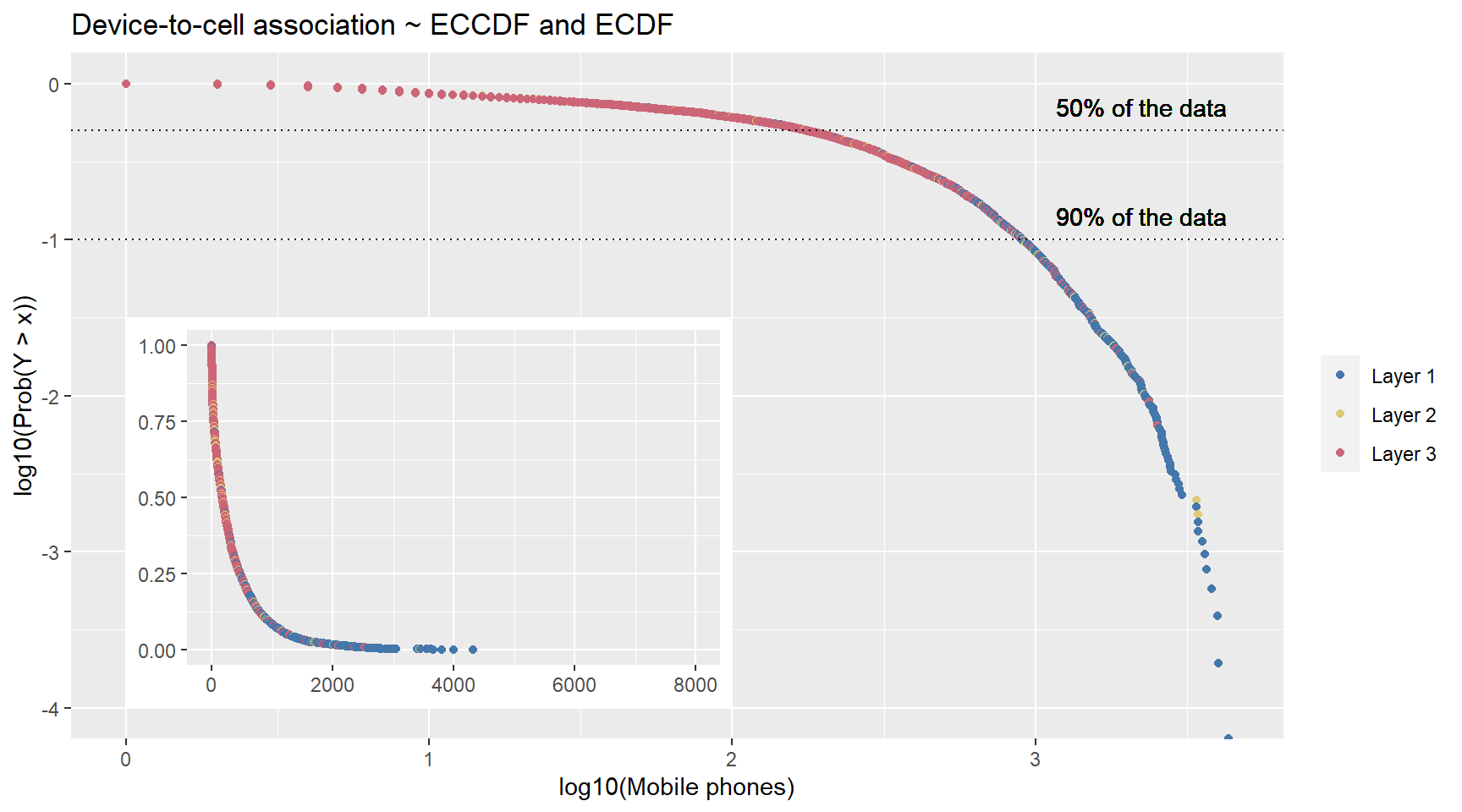
Figure 4.10: Mobile devices are predominately associated with Layer 1 antennas.
Once again, we use the ECCDF with log10 to better understand the distribution of the device-to-cell association. 50% of the devices is associated to the cells in the Rural layer. Furthermore, 90% of the devices are associated only to cells of layer 1 and layer 2, respectively Rural and Suburban. ONly 10% of the devices are associated also to the layer 3, which Urban.
Next we can specify the corresponding vector \(u\), which is of length of the unique number of tiles and contains the tile specific mobile phone population.
# u-vector
U.vec <- census.classified.final.sf %>%
  dplyr::select(internal.id, pop)

# saveRDS(U.vec, file = "C:/Users/Marco/Vysoká škola ekonomická v Praze/Tony Wei Tse Hung - YAY/working objects/U.vec.rds")
And finally, we can specify the final version of \(P\), which will serve as an oracle model later on. We will build multiple versions of \(P\) that will ease up processes with formatting. P.helper.geo is a long format version, which contains the columns internal.id, antenna.ID, weight.pij and the geometry of the tiles. P.helper which excludes the geometry. And P.mat which is a sparseMatrix object.
# sparse P matrix of device to cell
P.helper.geo <- dev.to.cell.classified %>%
  dplyr::select(internal.id, antenna.ID, weight.pij) %>%
  mutate_at(vars(c("internal.id", "antenna.ID")), factor)

# saveRDS(P.helper.geo, file = "C:/Users/Marco/Vysoká škola ekonomická v Praze/Tony Wei Tse Hung - YAY/working objects/P.helper.geo.rds")
# P.helper.geo <- readRDS(file = "C:/Users/Marco/Vysoká škola ekonomická v Praze/Tony Wei Tse Hung - YAY/working objects/P.helper.geo.rds")

# P.helper <- P.helper.geo %>%
#   st_drop_geometry()
#
# saveRDS(P.helper, file = "Vysoká škola ekonomická v Praze/Tony Wei Tse Hung - YAY/working objects/P.helper.rds")
# # P.helper.missing <- readRDS(file = "Vysoká škola ekonomická v Praze/Tony Wei Tse Hung - YAY/working objects/P.helper.missing.rds")


P.mat <- sparseMatrix(i = as.numeric(P.helper.geo$antenna.ID),
                      j = as.numeric(P.helper.geo$internal.id),
                      x = P.helper.geo$weight.pij,
                      dimnames = list(levels(P.helper.geo$antenna.ID), levels(P.helper.geo$internal.id)))


# saveRDS(P.mat, file = "C:/Users/Marco/Vysoká škola ekonomická v Praze/Tony Wei Tse Hung - YAY/working objects/P.mat.rds")
With the specification of \(P\), \(c\) and \(u\), we finalize our toy world generation. We are now able to use these objects as our ground truth. The next chapter will introduce four estimation techniques to model \(u\).