6.1 Evaluation of all estimates

We created 4 final estimates:

• Voronoi tessellation with tower locations as seeds

• Voronoi tessellation with coverage area locations (antennas) as seeds

• MLE uniform prior equal probability P.matrix after 1000 iterations

• MLE uniform prior oracle probability P.matrix after 1000 iterations

We will create an object, final.estimates, which contains all estimator results as well as the true population, pop, on the tile level.

census.classified.final.sf <- readRDS("C:/Users/Marco/Vysoká škola ekonomická v Praze/Tony Wei Tse Hung - YAY/working objects/census.classified.final.sf.rds")
voronoi.final.both <- readRDS("C:/Users/Marco/Vysoká škola ekonomická v Praze/Tony Wei Tse Hung - YAY/Estimates/Voronoi both/Voronoi.estimates.rds")
u.equal.selected <- readRDS("C:/Users/Marco/Vysoká škola ekonomická v Praze/Tony Wei Tse Hung - YAY/Estimates/u.equal.selected.rds")
u.oracle.selected <- readRDS("C:/Users/Marco/Vysoká škola ekonomická v Praze/Tony Wei Tse Hung - YAY/Estimates/u.oracle.selected.rds")

final.estimates <- voronoi.final.both %>% 
  left_join(u.equal.selected, by = "internal.id") %>% 
  left_join(u.oracle.selected, by = "internal.id") %>% 
  left_join(census.classified.final.sf, by = "internal.id") %>% 
  dplyr::select(internal.id, geometry, pop.area.kind, pop = pop.x, voronoi.est.antenna, voronoi.est.tower, mle.est.equal.1000 = u.equal.1000, mle.est.oracle.1000 = u.oracle.1000)

In the following we compare the distributions of the final estimates to the true distribution of the mobile phone density per tile. Significant variation can only be viewed in the tails of the distribution (ECCDF).

custom_ecdf_prep <- function(df, value) {
  data <- df %>% 
    mutate(pop.plot = value + 1) %>%  
    arrange(pop.plot) %>%  
    mutate(prob = 1 / n()) %>%  
    mutate(cum.prob = cumsum(prob)) %>%  
    mutate(cum.prob.comp = 1 - cum.prob) %>%  
    mutate(log10.cum.prob.comp = log10(cum.prob.comp)) %>% 
    mutate(log10.pop = log10(pop.plot)) %>%  
    mutate(cum.prob.comp = 1 - cum.prob)
  
  return(data)
}


# Creating the data frame we need to graph the eccdf 
dist.comp.helper <- final.estimates %>% 
  dplyr::select(-c(geometry, pop.area.kind)) %>% 
  pivot_longer(-internal.id, names_to = "estimator", values_to = "value") %>% 
  mutate(estimator = factor(estimator, levels = c("voronoi.est.tower", "voronoi.est.antenna", 
                                                  "mle.est.equal.1000", "mle.est.oracle.1000", "pop"))) %>% 
  mutate(value = round(value, 2)) %>% 
  split(.$estimator) %>% 
  map(~custom_ecdf_prep(.)) 

final.ECCDF.data <- dist.comp.helper %>% 
  map(~dplyr::select(., log10.cum.prob.comp, log10.pop)) %>%
  map(~mutate(., log10.cum.prob.comp = round(log10.cum.prob.comp, 3))) %>% # effective plot sample --> faster plotting excluding overplot
  map_dfr(~distinct(.), .id = "estimator")

final.ECDF.data <- dist.comp.helper %>% 
  map(~dplyr::select(., cum.prob.comp, pop.plot)) %>%
  map(~mutate(., cum.prob.comp = round(cum.prob.comp, 3))) %>% # effective plot sample --> faster plotting excluding overplot
  map_dfr(~distinct(.), .id = "estimator")

# Plot the ECCDF
est.names <- c("Voronoi ~ Tower", "Voronoi ~ Antenna", "MLE ~ Equal", "MLE ~ Oracle") 
ECCDF.estimates.plot <- final.ECCDF.data %>% 
  ggplot() + 
  geom_point(aes(x = log10.pop, y = log10.cum.prob.comp, color = estimator), size = 1) + 
  scale_color_ptol(breaks = c("voronoi.est.tower", "voronoi.est.antenna", "mle.est.equal.1000", "mle.est.oracle.1000", "pop"),
                   labels = c(est.names, "True Pop")) + 
  theme(legend.position = "bottom") +
  labs(title = "Estimator Comparison ~ ECCDF and ECDF", y = "Prob(Y > x)", x = "Mobile phones", color = "Estimator")

# plot the ecdf using ggplot
ECDF.estimates.plot <- final.ECDF.data %>%
  ggplot() + 
  geom_point(aes(x = pop.plot, y = cum.prob.comp, color = estimator)) + 
  scale_color_ptol(breaks = c("voronoi.est.tower", "voronoi.est.antenna", "mle.est.equal.1000", "mle.est.oracle.1000", "pop"),
                   labels = c(est.names, "True Pop"),
                   guide = F, expand = c(0, 0)) +
  xlim(0, 2000) +
  labs(y = "", x = "") +
  theme(plot.title = element_text(size = 10, face = "bold", hjust = 0.5),
        plot.subtitle = element_text(size = 9, hjust = 0.5),
        axis.title.x = element_blank(),
        axis.title.y = element_blank())

estimates.ECCDF.ECDF.plot <- ECCDF.estimates.plot +
  annotation_custom(ggplotGrob(ECDF.estimates.plot), 
                    xmin = 0, xmax = 1.5, 
                    ymin = -6, ymax = -3)

# saveRDS(estimates.ECCDF.ECDF.plot, "C:/Users/Marco/Vysoká škola ekonomická v Praze/Tony Wei Tse Hung - YAY/Estimates/Plot.files/estimates.ECCDF.ECDF.plot.rds") # save the plot as a rds file

estimates.ECCDF.ECDF.plot

In this section we want to further evaluate the 4 estimates by comparing them with different perspectives in mind to the actual true population. Each subsection defines the perspective-respective performance measure:

1. Geographical evaluation through the use of maps to show the final results of each estimation strategy

2. Statistical evaluation through the use of MAD and AAD metrics to compare the statistical accuracy of each estimation strategy.

6.1.1 Geographical Evaluation

For the geographical evaluation we use the following performance measure: The visual resemblance of fixed tile categories from the respective estimate and the actual true population on a map.

We basically build a map for every final estimate and compare it to the actual true population.

true.geo.eval.plot <- readRDS("~/OneDrive - Vysoká škola ekonomická v Praze/YAY/Estimates/Plot.files/true.pop_map.rds")

VT.geo.eval.plot <- readRDS("~/OneDrive - Vysoká škola ekonomická v Praze/YAY/Estimates/Plot.files/VT.estimate_map.rds")

true.geo.eval.plot = true.geo.eval.plot + theme(axis.text.x=element_text(angle=90, hjust=1))
VT.geo.eval.plot = VT.geo.eval.plot + theme(axis.text.x=element_text(angle=90, hjust=1))

true.geo.eval.plot
VT.geo.eval.plot

# plot_grid(true.geo.eval.plot, VT.geo.eval.plot, labels = "Fig. 14 Comparing Voronoi tower estimate", label_size = 12,align = "hv", hjust = -0.1)

VA.geo.eval.plot <- readRDS("~/OneDrive - Vysoká škola ekonomická v Praze/YAY/Estimates/Plot.files/VA.estimate_map.rds")

VA.geo.eval.plot = VA.geo.eval.plot + theme(axis.text.x=element_text(angle=90, hjust=1))

true.geo.eval.plot
VA.geo.eval.plot

#plot_grid(true.geo.eval.plot, VA.geo.eval.plot, labels = "Fig. 15 Comparing Voronoi antenna estimate", label_size = 12,align = "hv", hjust = -0.1)

# MLE.equal.geo.eval.plot <- readRDS("Estimates/Plot.files/MLE.oracle.estimate_map.rds")
# animate(MLE.equal.geo.eval.plot, fps = 10)

# plot_grid(true.geo.eval.plot, MLE.equal.geo.eval.plot,
#           labels = "Comparing MLE equal P.matrix estimate", label_size = 12,
#           align = "hv", hjust = -0.1)

# MLE.true.geo.eval.plot <- readRDS("Estimates/Plot.files/MLE.oracle.estimate_map.rds")
# MLE.true.geo.eval.plot <- animate(MLE.true.geo.eval.plot, fps = 10)
# 
# 
# plot_grid(true.geo.eval.plot, MLE.true.geo.eval.plot,
#           labels = "Comparing MLE true P.matrix estimate", label_size = 12,
#           align = "hv", hjust = -0.1)


knitr::include_graphics("https://raw.githubusercontent.com/R-ramljak/MNO_Eurostat/master/Gifs/MLE.equal.estimate_map_new.gif")
knitr::include_graphics("https://raw.githubusercontent.com/R-ramljak/MNO_Eurostat/master/Gifs/MLE.oracle.estimate_map_new.gif")

6.1.2 Statistical/Distributional Evaluation

In order to actually compare the numerical resemblance between the estimates and the actual true population we introduce two discrepancy performance measures.

• Average Absolute Discrepancy (AAD): \(D_{avg}(u,v) = \frac{1}{U}\sum_{j = 1}^{J} |u_{j} - v_{j}|\)

• Maximum Absolute Discrepancy (MAD): \(D_{max}(\textbf{u,v}) \overset{\underset{\mathrm{def}}{}}{=} \sum_{\mathit{j = 1}}^{\mathit{J}}\left | u_{j} - v_{j} \right |\)

# Average Absolute Discrepancy and Maximum Absolute Discrepancy Calculation:
stat.eval <- final.estimates %>%
  mutate_at(vars(contains("est.")), list(diff = ~abs(pop - .))) %>% 
  summarise_at(vars(contains("diff")), list("aad" = ~sum(.) / sum(pop),
                                            "mad" = ~sum(.))) %>% 
  pivot_longer(-c(), names_to = "type", values_to = "value") %>% 
  separate(type, into = c("estimator", "type"), sep = "_diff_") %>% 
  mutate(estimator = factor(estimator, levels = c("voronoi.est.tower", "voronoi.est.antenna", 
                                                  "mle.est.equal.1000", "mle.est.oracle.1000"))) 

est.names <- c("Voronoi ~ Tower", "Voronoi ~ Antenna", "MLE ~ Equal", "MLE ~ Oracle") 

# aad plot
aad.comp.plot <- stat.eval %>%
  filter(type == "aad") %>% 
  ggplot(aes(x = estimator, y = value, fill = estimator)) + 
  geom_bar(stat = "identity") + 
    geom_text(aes(x = estimator, y = value, label = round(value, 2)), 
            hjust = 1.3, color = "white", size = 4) +
  labs(x = "", y = "Average Absolute Discrepancy", fill = "", title = "Estimator Comparison ~ AAD") + 
  theme(legend.position = "bottom") +
  scale_x_discrete(breaks = c("voronoi.est.tower", "voronoi.est.antenna", "mle.est.equal.1000", "mle.est.oracle.1000"), 
                  labels = est.names) +
  scale_fill_ptol(breaks = c("voronoi.est.tower", "voronoi.est.antenna", "mle.est.equal.1000", "mle.est.oracle.1000"), 
                  labels = est.names) +
  coord_flip()

# saveRDS(aad.comp.plot, file = "C:/Users/Marco/Vysoká škola ekonomická v Praze/Tony Wei Tse Hung - YAY/estimation plots/aad.comp.plot.rds")

# mad plot
mad.comp.plot <- stat.eval %>%
  filter(type == "mad") %>% 
  ggplot(aes(x = estimator, y = value, fill = estimator)) + 
  geom_bar(stat = "identity") + 
  geom_text(aes(x = estimator, y = value, label = round(value, 0)), 
            hjust = 1.3, color = "white", size = 4) +
  labs(x = "", y = "Maximum Absolute Discrepancy", fill = "", title = "Estimator Comparison ~ MAD") + 
  theme(legend.position = "bottom") +
  scale_x_discrete(breaks = c("voronoi.est.tower", "voronoi.est.antenna", "mle.est.equal.1000", "mle.est.oracle.1000"), 
                  labels = est.names) +
  scale_fill_ptol(breaks = c("voronoi.est.tower", "voronoi.est.antenna", "mle.est.equal.1000", "mle.est.oracle.1000"), 
                  labels = est.names) +
  coord_flip()

# saveRDS(mad.comp.plot, file = "C:/Users/Marco/Vysoká škola ekonomická v Praze/Tony Wei Tse Hung - YAY/estimation plots/mad.comp.plot.rds")

aad.comp.plot
mad.comp.plot

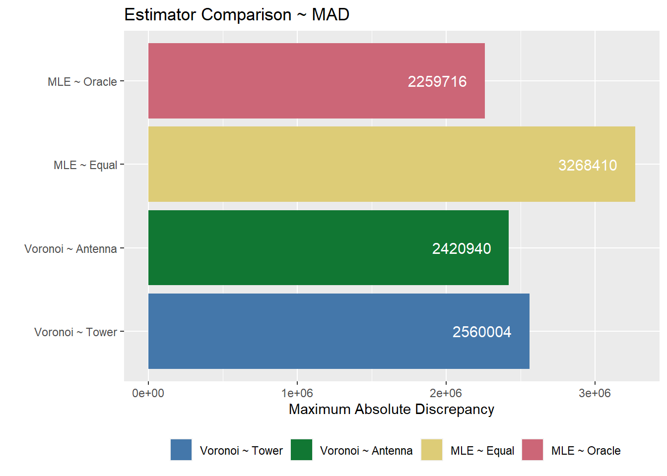
Figure 6.1: …

By calculating the two discrepancy measures, we can then evaluate the overall performance for each type of estimation. In general, the Voronoi estimates result in less discrepancy compared to both of the MLE estimates. Between the two MLE estimates, the true population matrix has a lower discrepancy than the equal population matrix. Between the two Voronoi estimates, the Voronoi estimation by antennas has a lower discrepancy than the Voronoi estimation by towers.

6.1.3 Kantorovich-Wasserstein Distance (KWD)

The KWD is different such that it takes in consideration of the spatial component which was not considered by the previous metrics. Thus it is safe to say that it is a more holistic assessment of the different estimation strategies.

kwd.helper.est.1x1 <- final.estimates %>% 
  st_sf(sf_column_name = "geometry", crs = 3035) %>% 
  mutate(lon = map_dbl(geometry, ~st_centroid(.x)[[1]]),
         lat = map_dbl(geometry, ~st_centroid(.x)[[2]])) %>% 
  st_drop_geometry()
# saveRDS(kwd.helper.est.1x1, "C:/Users/Marco/Vysoká škola ekonomická v Praze/Tony Wei Tse Hung - YAY/working objects/kwd.helper.est.rds")

coordinates.1x1 <- kwd.helper.est.1x1 %>% 
  select(lon, lat) %>% 
  as.matrix()

weights.1x1 <- kwd.helper.est.1x1 %>% 
  select(pop, voronoi.est.tower, voronoi.est.antenna, mle.est.equal.1000, mle.est.oracle.1000) %>% 
  as.matrix()

kwd.final.1x1 <- compareOneToMany(coordinates, weights, L = 2, recode = TRUE)
cat("runtime:", kwd.final.1x1$runtime, " distance:", kwd.final.1x1$distance, " nodes:", kwd.final.1x1$nodes, " arcs:", kwd.final.1x1$arcs, "\n")

saveRDS(kwd.final.1x1, "C:/Users/Marco/Vysoká škola ekonomická v Praze/Tony Wei Tse Hung - YAY/Evaluation/kwd.final.1x1.rds")

# 4x4 scale

census.4x4 <- census.classified.final.sf %>% 
  dplyr::select(internal.id, pop) %>% 
  st_make_grid(cellsize = 400)

kwd.helper.est.4x4 <- final.estimates %>% 
  st_sf(sf_column_name = "geometry", crs = 3035) %>% 
  aggregate(by = census.4x4, FUN = sum, join = st_contains) %>% 
  mutate(lon = map_dbl(geometry, ~st_centroid(.x)[[1]]),
         lat = map_dbl(geometry, ~st_centroid(.x)[[2]])) %>% 
  st_drop_geometry()


coordinates.4x4 <- kwd.helper.est.4x4 %>% 
  select(lon, lat) %>% 
  as.matrix()

weights.4x4 <- kwd.helper.est.4x4 %>% 
  select(pop, voronoi.est.tower, voronoi.est.antenna, mle.est.equal.1000, mle.est.oracle.1000) %>% 
  as.matrix()

kwd.final.4x4 <- compareOneToMany(coordinates.4x4, weights.4x4, L = 2, recode = TRUE)
cat("runtime:", kwd.final.4x4$runtime, " distance:", kwd.final.4x4$distance, " nodes:", kwd.final.4x4$nodes, " arcs:", kwd.final.4x4$arcs, "\n")

# saveRDS(kwd.final.4x4, "C:/Users/Marco/Vysoká škola ekonomická v Praze/Tony Wei Tse Hung - YAY/Evaluation/kwd.final.4x4.rds")

# kwd plot
kwd.eval <- tibble(estimator = c("voronoi.est.tower", "voronoi.est.antenna", "mle.est.equal.1000", "mle.est.oracle.1000"), 
                   kwd.1x1 = kwd.final.1x1$distance,
                   kwd.4x4 = kwd.final.4x4$distance * 4) %>% # rescaling according to scale 
  pivot_longer(-estimator, names_to = "kwd.scale", values_to = "value") %>% 
  mutate(estimator = factor(estimator, levels = c("voronoi.est.tower", "voronoi.est.antenna", 
                                                  "mle.est.equal.1000", "mle.est.oracle.1000"))) 

kwd.plot <- kwd.eval %>% 
  ggplot(aes(x = kwd.scale, y = value, fill = estimator)) + 
  geom_bar(stat = "identity", position = "dodge") + 
  geom_text(aes(x = kwd.scale, y = value, label = round(value, 2)), 
            position = position_dodge(0.9), hjust = 1.3, color = "white", size = 4) +
  labs(x = "", y = "KWD", fill = "Estimator", title = "Estimator Comparison ~ KWD, L = 2") + 
  theme(legend.position = "bottom") +
  scale_x_discrete(breaks = c("kwd.4x4", "kwd.1x1"), 
                  labels = c("KWD ~ 4x4", "KWD ~ 1x1")) +
  scale_fill_ptol(breaks = c("voronoi.est.tower", "voronoi.est.antenna", "mle.est.equal.1000", "mle.est.oracle.1000"), 
                  labels = est.names) +
  coord_flip()

# saveRDS(kwd.plot, file = "C:/Users/Marco/Vysoká škola ekonomická v Praze/Tony Wei Tse Hung - YAY/estimation plots/kwd.plot.rds")

kwd.plot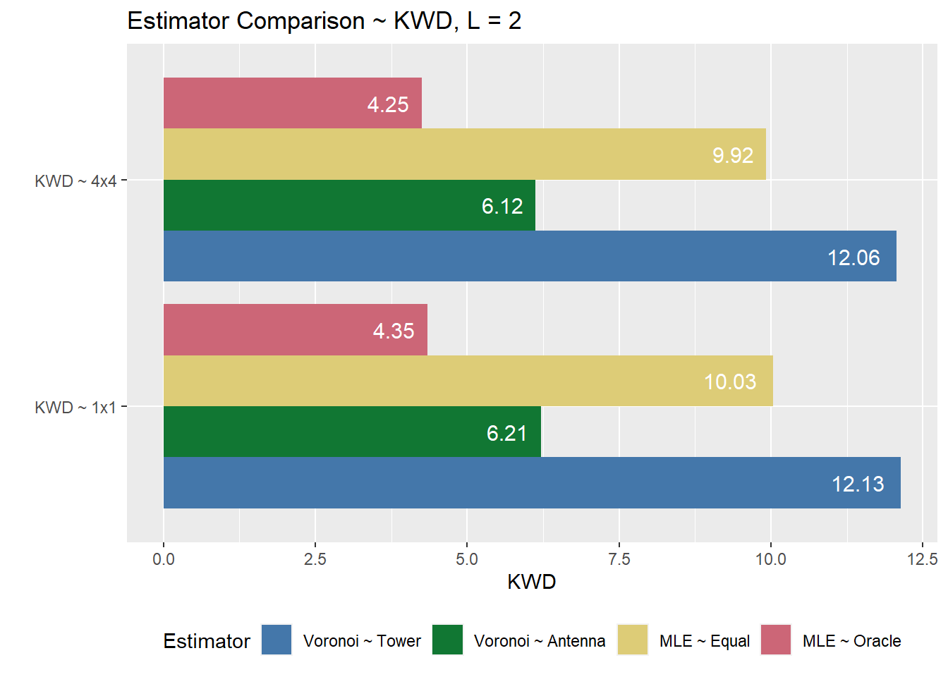

Figure 6.2: …

# ggsave("C:/Users/Marco/Vysoká škola ekonomická v Praze/Tony Wei Tse Hung - YAY/estimation plots/kwd.plot.png", kwd.plot, device = "png")