Chapter 1 Introduction to Research and Data
Welcome to the wonderful world of data analysis! Here, depending on how your instructor organizes your course, you will learn the “nuts and bolts” of doing data analysis, including topics ranging from when and how to use both relatively simple and somewhat more complicated statistics, to the important role of different types of graphics, to how to write relatively simple computer commands that connect you to the data you need for your analysis. This chapter introduces several terms and concepts that provide a framework for easing into these and other topics related to political and social data analysis.
Data Analysis or Statistics?
This textbook provides an introduction to data analysis, and should not be confused with a statistics textbook. Technically, it is not possible to separate data analysis from statistics, as statistics is a field of study that emerged specifically for the purpose of providing techniques for analyzing data. In fact, with the exception of this chapter, most of the material in this book addresses the use of statistical methods to analyze political and social outcomes; but that is different from a focus on statistics for the sake of learning statistics. Most straight-up texts on statistics highlight the sometimes abstract, mathematical foundations of statistical techniques, with less emphasis on concrete applications. This textbook, along with most undergraduate books on data analysis, focuses much more on concrete applications of statistical methods that facilitate the analysis of political and social outcomes.
Some students may be breathing a sigh of relief, thinking, “Oh good, there’s no math or formulas!” Not quite. The truth of the matter is that while a lot of the math underlying the statistical techniques can be intimidating and off-putting to people with a certain level of math anxiety (including the author of this book!), some of the key formulas for calculating statistics are very intuitive, and taking time to focus on them (even at a surface level) helps students gain a solid understanding of how to interpret statistical findings. So, while there is not much math in the pages that follow, there are a few statistical formulas, sometimes with funny-looking Greek letters. The main purpose of presenting formulas, though, is to facilitate understanding and to make statistics more meaningful to the reader. If you can add, subtract, divide, multiply, and follow instructions, the “math” in this book should not present a problem.
Uses of Data Analysis
Contemporary society is swimming in data, and examples of data analysis abound. In fact, if you look at the world around you, you will find plenty of applications of data analysis, encompassing everything from sports analytics (including some of the silly statistics reported during broadcasts of sportint events), to discussions of the prevalence of COVID-19 and the effectiveness of vaccines, to monthly reports of inflation or quarterly updates of economic growth, to weather forecasts, to analyzing the impact of public policies, to models used to select jurors, and many more interesting applications.
Whatever the substantive focus, data analysis can take a number of different forms. Sometimes the goal of data analysis is simply to describe something, to show how measures of some outcomes are distributed. This is referred to as descriptive analysis, and can play a very interesting and useful in understanding the state of the world. One example of this that you may be most familiar with is media coverage of public opinion polls, especially those related to elections. By reporting the percent of voters who intend to vote for one candidate or the other, media outlets are describing what political preferences look like at the time of the poll.
Descriptive analysis can take many different forms, including reporting simple results, as in the current polling example, or reporting more advanced statistics that help the clarify how the outcomes are distributed, or perhaps using any number of graphing tools that visualize the outcomes. Descriptive analysis is the focus of the first several chapters of this book and makes important contributions to many of the other chapters.
Other times, the goal of research is to not just describe outcomes but also to explain why or how those outcomes occurred. This is referred to as explanatory analysis. For instance, when reporting the results of an election poll, you might sometimes see media outlets focus on how characteristics such as racial/ethnic identity, sex, ideology, or issue positions are related to which candidates people support. In this sort of very simple form, there is not a lot of difference between descriptive and explanatory analysis, as the goal is to describe what sorts of people support the candidates. A more formal type of explanatory analysis that involves developing and testing specific hypotheses about how outcomes on some variables are influenced by outcomes on others is discussed in the next section and given much fuller treatment beginning in Chapter 8.
Whether researchers are interested in descriptive or explanatory analysis, one important aspect of all forms of data analysis is related to finding valid and reliable ways to develop (usually) quantitative measures of the outcomes of interest. This concern with measurement is central to all forms of empirical political and social data analysis. Issues related to measurement are covered in the next section and are also interwoven into some of the later chapters.
The Research Process
Though the emphasis in this book is squarely on data analysis, that is just one important part of the broader research enterprise. In fact, data analysis on its own is not very meaningful, especially if explanatory analysis is the focus of the research. Instead, for data analysis to produce meaningful and relevant results, it must take place in the context of a set of expectations and be based on a host of decisions related to those expectations.
Social science research can be thought of as a process, where there is a beginning and an end, although it is also possible to imagine the process as cyclical and ongoing. What is presented below is an idealized version of the research process. There are a couple of important things to understand about this description. First, this process is laid out in four very broadly defined categories for ease of understanding. The text elaborates on a lot of important details that should not be skipped. Second, in the real world of the research there can be a bit of jumping around from one part of the process to another, not always in the order shown below. Finally, this is just one of many different ways of describing the research process. In fact, if you consult ten different books on research methods in the social sciences, you will probably find ten somewhat different depictions of the research process. Having said this, though, at least in points of emphasis, all ten depictions should have a lot in common. The major parts of this process are presented in Figure 1.1.
[Figure******** 1.1 ********about here]
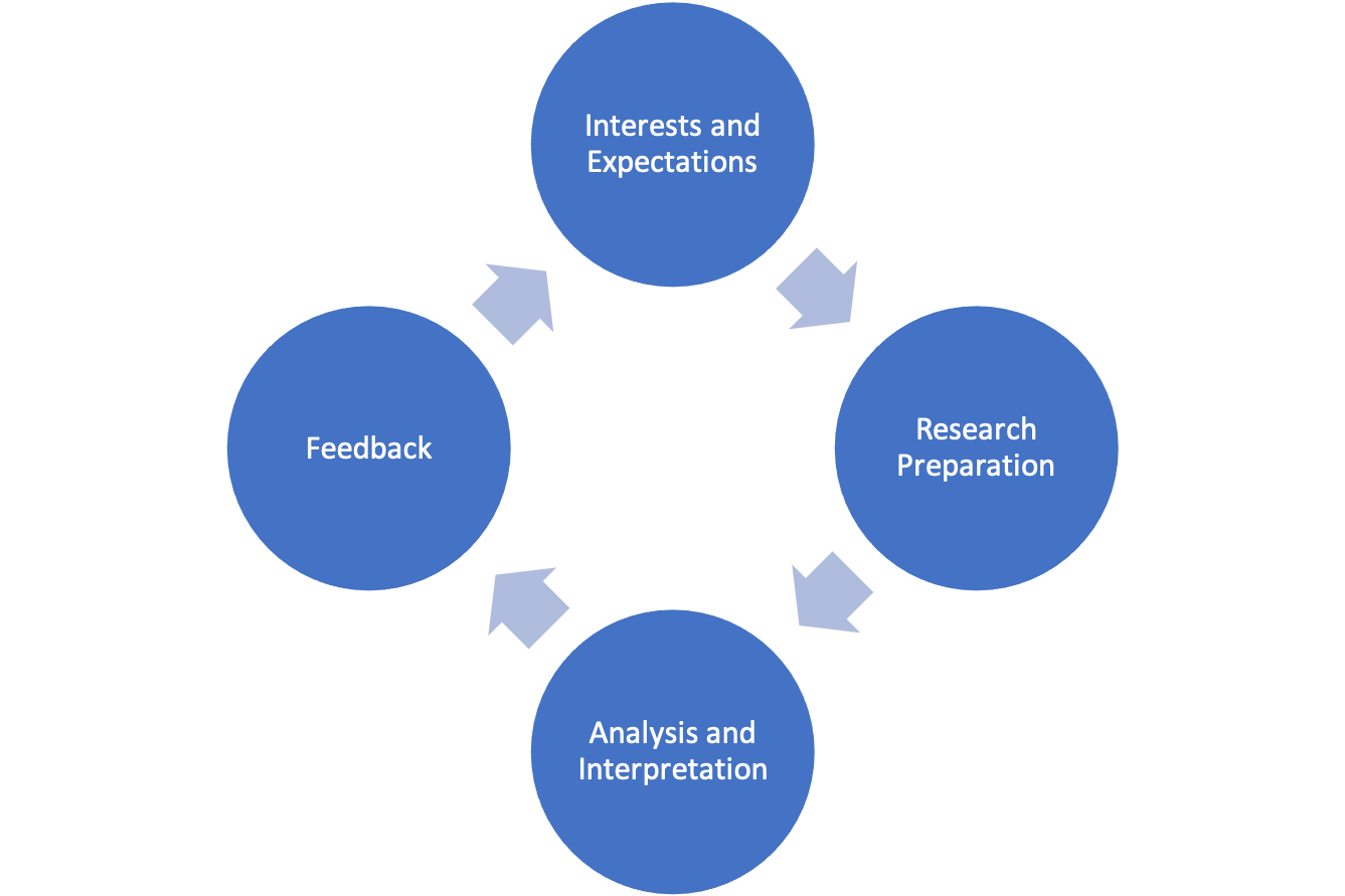
Figure 1.1: An Idealized Description of the Research Process
Interests and Expectations
The foundation of the research process is research interests or research ideas. College students are often asked to write research papers and one of the first parts of the writing assignment is to identify their research interests or, if they are a bit farther along, their research topic. Students frequently start with something very broad, perhaps, “I want to study elections,” or something along the lines of “LGBTQ rights.” This is good to know, but it is still too overly general to be very helpful. What is it about elections or LGBTQ rights that you want to know? The key to really kicking things off is to narrow the focus to a more useful research question. Maybe a student interested in elections has observed that some presidents are re-elected more easily than others, and settles on a more manageable goal, explaining the determinants of incumbent success in presidential elections. Maybe the student interested in LGBTQ rights has observed that some states offer several legal protections for LGBTQ residents, while other states do not. In this case, the student might limit their research interest to explaining variation in LGBTQ rights across the fifty states. The key here is to move from a broad subject area to a narrower research question that gives some direction to the rest of the process.
Theory
Still, even if a researcher has narrowed their research interest to a more manageable topic, they need to do a bit more thinking before they can really get started; they need a set of expectations to guide their research. In the case of studying sources of incumbent success, for instance, it is still not clear where to begin. Students need to think about their expectations. What are some ideas about the things that might be related to incumbent success? Do these ideas make sense? Are they reasonable expectations? What theory is guiding your research?
“Theory” is one of those terms whose meaning we all understand at some level and perhaps even use in everyday conversations (e.g., “My theory is that…”), but it has a fairly specific meaning in the research process. In this context, theory refers to a set of logically connected propositions (or ideas/statements/assumptions) that we take to be true and that, together, can be used to explain a given outcome or set of outcomes. Think of a theory as a rationale or plausible framework for testing ideas about things that might explain the outcomes of interest.
As an example, a theory of retrospective voting can be used to explain support and opposition to incumbent presidents. The retrospective model was developed in part in reaction to findings from political science research that showed that U.S. voters did not know or care very much about ideological issues and, hence, could not be considered “issue voters.” Political scientist Morris Fiorina’s work on retrospective voting countered that voters don’t have to know a lot about issues or candidate positions on issues to be issue voters.1 Instead, he argued that the standard view of issue voting is too narrow and a theory based retrospective issues does a better job of describing the American voter. Some of the key tenets of the retrospective model are:
Elections are referendums on the performance of the incumbent president and their party;
Voters don’t need to understand or care about the nuances of foreign and domestic policies of the incumbent president to hold their administration accountable;
Voters only need to be aware of the results of those policies, i.e., have a sense of whether things have gone well on the international (war, trade, crises, etc.) and domestic (economy, crimes, scandals, etc.) fronts;
When times are good, voters are inclined to support the incumbent party; when times are bad, they are less likely to support the incumbent party.
This is an explicitly reward-punishment model. It is referred to as retrospective voting because the emphasis is on looking back on how things have turned out under the incumbent administration rather than comparing details of policy platforms to decide if the incumbent or challenging party has the best plans for the future.
Hypotheses
The next step in this part of the research process is developing hypotheses that logically flow from the theory. A hypothesis is speculation about the state of the world. Research hypotheses are based on theories and usually assert that variations in one variable are associated with, result in, or cause variation in another variable. Typically, hypotheses specify an independent variable and a dependent variable. Independent (explanatory) variables, often represented as X, are best thought of as the variables that influence, or shape outcomes in other variables. They are referred to as independent because we are not assuming that their outcomes depend on the values of other variables. Dependent (response) variables, often represented as Y, measure the thing we want to explain. These are the variables that we think are affected by the independent variables. One short-cut to recalling this is to remember that the outcome of the dependent variable depends upon the outcome of the independent variable.
Based on the theory of retrospective voting, for instance, it is reasonable to hypothesize that economic prosperity is positively related to the level of popular support for the incumbent president and their party. Support for the president should be higher when the economy is doing well than when it is not doing well. In social science research, hypotheses sometimes are set off and highlighted separately from the text, just so it is clear what they are:
H1: Economic prosperity is positively related to the level of popular support for the incumbent president and their party. Support for the president should be higher when the economy is doing well than when it is not doing well.
In this hypothesis, the independent and dependent variables are represented by two important concepts, economic prosperity and support for the incumbent president, respectively. Concepts are broad, abstract ideas that define theoretically relevant phenomena and help us understand the meaning of the theory a bit more clearly. But while concepts such as these help us understand the expectations embedded in the hypothesis, they are sufficiently broad and abstract that we are not quite ready to analyze the data.
Research Preparation
In this stage of the research process, a number of important decisions need to be made regarding the measurement of key concepts, the types of data that will be used, and how the data will be obtained. The hypothesis developed above asserts that two concepts–economic prosperity and support for the incumbent president–are related to each other. When you hear or read the names of these concepts, you probably generate a mental image that helps you understand what they mean. However, they are still a bit too abstract to be useful from a measurement perspective.
Measurement Issues
What we need to do is move from abstract concepts to operational variables–concrete, tangible, measurable representations of the concepts. How are these concepts going to be represented when doing the research? There are a number of ways to think about measuring these concepts (see Table 1.2). If we take “economic prosperity” to mean something like how well the economy is doing, we might decide to use some broad-based measure, such as percentage change in the gross domestic product (GDP) or percentage change in personal income, or perhaps the unemployment rate at the national level. We could also opt for a measure of perceptions of the state of the economy, relying on survey questions that ask individuals to evaluate the state of the economy, and there are probably many other ways you can think of to measure economic prosperity. Even after deciding which measure or measures to use, there are still decisions to be made. For instance, let’s assume we decide to use change in GPD as a measure of prosperity. We still need to decide over what time period we need to measure change. GDP growth since the beginning of the presidential term? Over the past year? The most recent quarter? It’s possible to make good arguments for any of these choices.
[Tbl 1.2 about here]
Table 1.2. Possible Operational Measures of Key Concepts
| Concept | Operational Variables |
|---|---|
| Economic Prosperity | GDP change, income change, economic perceptions, unemployment, etc. |
| Incumbent Support | Approval rating, presidential elections, congressional elections, etc. |
The same decisions have to be made regarding a measure of incumbent support. In this case, we might use polling data on presidential approval, presidential election results, or perhaps support for the president’s party in congressional elections. The point is that before you can begin gathering relevant data, you need to know how the key variables are being measured. In the example used here, it doesn’t require much effort to figure out how to operationalize the concepts that come from the hypotheses, but that is not always the case (think about measuring concepts such as power, justice, equality, fairness).
Table 1.2 also lists potential indicators of support for the incumbent president: presidential approval and election results. Presidential approval is based on responses to survey questions that ask if respondents approve or disapprove of the way the president is handling their job, and presidential election results are, of course, an official forum for registering support for the president (relative to their challenger) at the ballot box. Likewise, party gains and losses in congressional elections can be taken as an indicator of the level of support for the president’s party.
There are two very important concerns at the measurement stage: Validity and Reliability. The primary concern with validity is to make sure you are measuring what you think you are measuring. You need to make sure that the operational variables are good representations of the concepts. It’s tough to be certain of this, but one important, albeit imprecise, way to assess the validity of a measure is through its face validity. By this we mean, on its face, does this operational variable make sense as a measure of the underlying concept? If you have to work hard to convince yourself and others that you have a valid measure, then you probably don’t.
For reliability, the concern is with consistency. Here the question is whether you would get the same (or nearly the same) results if you measured the concept at different points in time, or across different (but similarly drawn) samples. So, for instance, in the case of measuring presidential approval, you would expect that outcomes of polls used do not vary widely from day to day and that most polls taken at a given point in time would produce similar results.
Data Gathering
Once a researcher has determined how they intend to measure the key concepts, they must find the data. Sometimes, a researcher might find that someone else has already gathered data they can use for their project. For instance, researchers frequently rely upon regularly occurring, large-scale surveys of public opinion that have been gathered for extended periods of time, such as the American National Election Study (ANES), the General Social Survey (GSS), or the Cooperative Election Study (CES). These surveys are based on large, scientifically drawn samples and include hundreds of questions on topics of interest to social scientists. Using data sources such as these is referred to as secondary data analysis.
Even when researchers are putting together their own data set, they frequently use secondary data. For instance, to test the hypotheses discussed above, a researcher may want to track election results and some measure of economic activity, economic growth. These data do not magically appear. Instead, the researcher has to put on their thinking cap and figure out where they can find sources for these data. As it happens, election results can be found at David Leip’s Election Atlas (https://uselectionatlas.org), and the economic data can be found at the Federal Reserve Economic Data website (https://fred.stlouisfed.org) and other government sites, though it takes a bit of poking around to actually find the right information.
Even after figuring out where to get their data, researchers still have several important decisions to make. Sticking with the retrospective voting hypothesis, if the focus is on national outcomes of U.S. presidential elections, there are a number of questions that need to be answered. In what time period are we interested? All elections? Post-WWII elections? How shall incumbent support be measured? Incumbent party percent of the total vote or percent of the two-party vote? If using the growth rate in GDP, over what period of time? Researchers need to think about these types of questions before gathering data.
As you can tell, measurement decisions are important and can be complicated to resolve. Time spent here, however, is almost guaranteed to deliver substantial payoffs further down the research process.
Data Analysis and Interpretation
Assuming a researcher has gathered appropriate data for testing their hypotheses and that the data have been coded in such a way that they are suitable to the task (more on this in the next chapter), the researcher can now subject the hypothesis to empirical scrutiny. By this, I mean that they can compare the state of the world as suggested by the hypothesis to the actual state of the world, as represented by the data gathered by the researcher. Generally, to the extent that the relationship between variables stated in the hypothesis resembles the relationship between the operational variables in the real world, then there is support for the hypothesis. If there is a significant disconnect between expectations from the hypothesis and the findings in the data, then there is less support for the hypothesis. Hypothesis testing is a lot more complicated than this, as you will see in later chapters, but for now let’s just think about it as comparing the hypothetical expectations to patterns in data.
Most of the rest of this book explores many different methods you can use to evaluate your hypotheses, some more appropriate than others, depending on the your research goals and the type of data you are using. Researchers are typically interested in two things, the strength of the relationship and the level of confidence in the findings. By “strength of the relationship” we mean how closely outcomes on the dependent and independent variables track with each other. For instance, if there is a clear and consistent tendency for incumbent presidents to do better in elections when the economy is doing well than when it is in a slump, then the relationship is probably pretty strong. If there is a slight tendency for incumbent presidents to do better in elections when the economy is doing well than when it is in a slump, then the relationship is probably weak.
Figure 1.2 provides a hypothetical example of what weak and strong relationships might look like, using generic independent and dependent variables. The scatterplot (you’ll learn much more about these in Chapter 14) on the left side illustrates a weak relationship. The first thing to note is that the pattern is not very clear; there is a lot of randomness to it, and, without the solid line in the data points, which summarizes the trend in the data and tilts upward slightly, it would be hard to discern that there is weak positive relationship in the graph. The best way to appreciate how weak the pattern is on the left side is to compare it with the pattern on the right side, where you don’t have to look very hard to notice a stronger trend in the data. In this case, there is a clear tendency for high values on the independent variable to be associated with high values on the dependent variable, indicating a strong, positive relationship.
[Figure******** 1.2 ********about here]
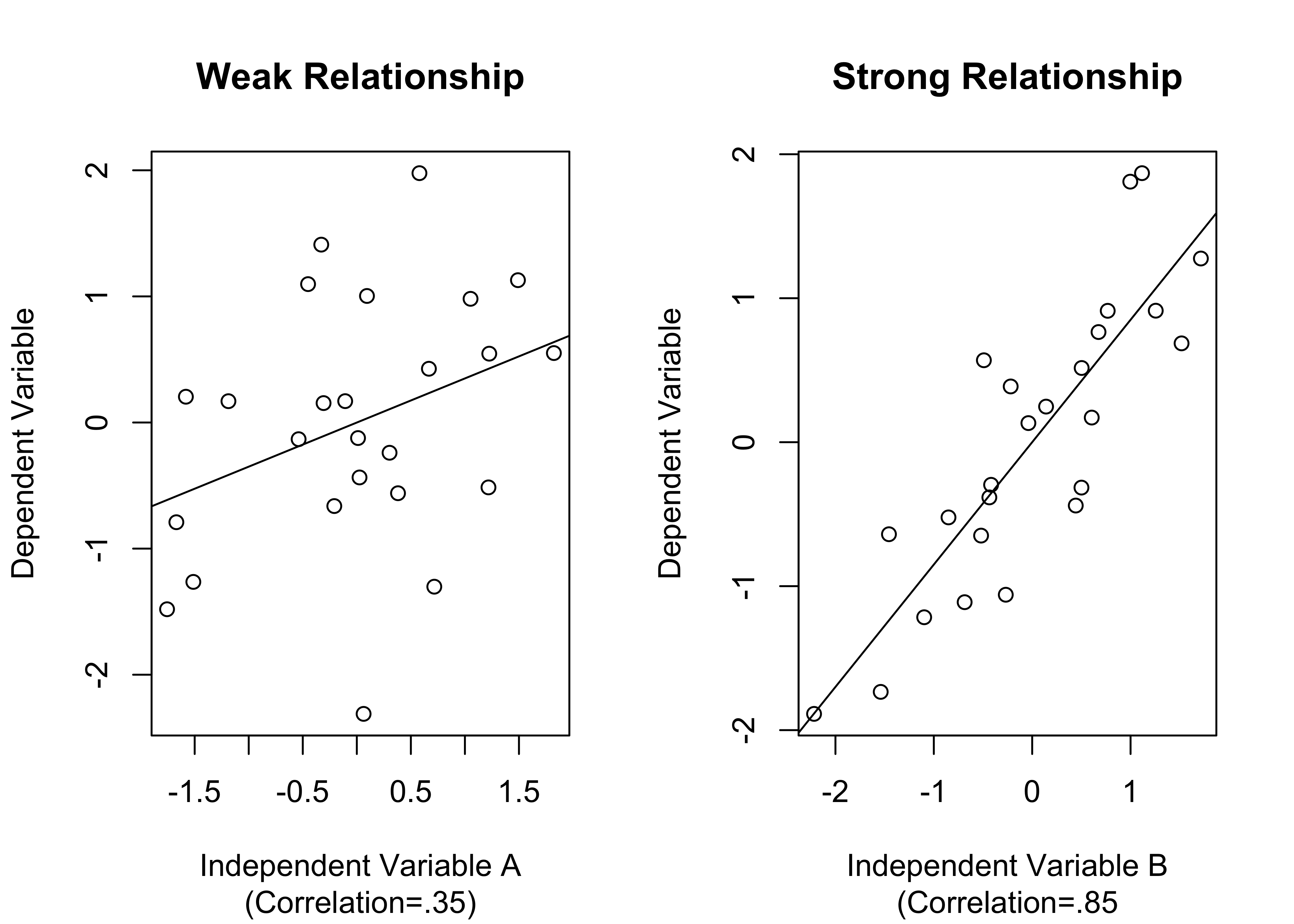
Figure 1.2: Simulated examples of Strong and Weak Relationships
Figure 1.2 provides a good example of data visualization, a form of presentation that can be a very important part of communicating research results. The idea behind data visualization is to display research findings graphically, primarily to help consumers of research contextualize and understand the findings.
To appreciate the importance of visualization, suppose you do not have the scatterplots shown above but are instead presented with the correlations in the figure (.35 for 85). These correlations are statistics that summarize how strong the relationships are, with values close to 0 meaning there is not much of a relationship, and values closer to 1 indicating strong relationships (much more on this and scatterplots in Chapter 14). If you had these statistics but no scatterplots, you would understand that Independent Variable B is more strongly related to the dependent variable than Independent Variable A is, but you might not fully appreciate what this means in terms of the predictive capacity of the two independent variables. The scatterplots help with this a lot.
At the same time, while the information in scatterplots gives you a clear intuitive impression of the differences in the two relationships, you can’t be very specific about how much stronger the relationship is for Independent Variable B without more precise information such as the correlation coefficients. Most often, the winning combination for communicating research results is some mix of statistical findings and data visualization.
In addition to measuring the strength of relationships, researchers also focus on their level of confidence in the findings. This is a key part of hypothesis testing and will be covered in much greater detail later in the book. The basic idea is that we want to know if the evidence of a relationship is strong enough that we can rule out the possibility that it occurred due to chance, or perhaps to measurement issues. Usually, especially with large samples, researchers can have a high level of confidence in strong relationships. However, weak relationships, especially those based on a small number of cases, do not inspire confidence (for instance, Independent Variable A in Figure 1.2). This may be a bit confusing at this point, but good research will distinguish between confidence and strength when communicating results. This point is emphasized later, beginning in Chapter 10.
One of the most important parts of this stage of the research process is the interpretation of the results. The key point to get here is that the statistics and visualizations do not speak for themselves. It is important to understand that knowing how to type in computer commands and get statistical results is not very helpful if you can’t also provide a coherent, substantive explanation of the results. Bottom line: Use words!
Typically, interpretations of statistical results focus on how well the findings comport with the expectations laid out in the hypotheses, paying special attention to both the strength of the relationships and the level of confidence in the findings, as discussed above. A good discussion of research findings will also acknowledge potential limitations to the research, whatever those may be.
By way of example, let’s look at a quick analysis of the relationship between economic growth and presidential support. To analyze this relationship, I gathered data on the percentage change in real GDP per capita during the first three quarters of the election year and the incumbent presidential party candidate’s percent of the two-party national popular vote in U.S. elections (presidential support), from 1948 to 2020. Note that these variables are concrete measures of abstract concepts (economic prosperity and presidential support) that flow from the theory of retrospective voting discussed earlier in this chapter.
An important linkage between data gathering and data analysis is organizing the data into a usable format. You will learn more about this in Chapter 2, but in the meantime, Table 1.3 provides you with a look at how the data are organized for this analysis.
[Tab 1.3 about here]
Table 1.3 Data for Testing the Retrospective Voting Hypothesis
| year | vote | gdpchng |
|---|---|---|
| 1948 | 52.4 | 1.03 |
| 1952 | 44.6 | 2.93 |
| 1956 | 57.8 | 1.00 |
| 1960 | 49.9 | -2.80 |
| 1964 | 61.3 | 1.93 |
| 1968 | 49.6 | 2.07 |
| 1972 | 61.8 | 4.17 |
| 1976 | 48.9 | 1.27 |
| 1980 | 44.7 | -1.19 |
| 1984 | 59.2 | 2.84 |
| 1988 | 53.9 | 2.53 |
| 1992 | 46.5 | 2.07 |
| 1996 | 54.6 | 2.69 |
| 2000 | 50.2 | 1.80 |
| 2004 | 51.2 | 2.00 |
| 2008 | 46.7 | -2.87 |
| 2012 | 52 | 0.14 |
| 2016 | 51.1 | 0.96 |
| 2020 | 47.7 | -1.52 |
The relationship between change in GDP and vote share for the incumbent party is shown below, in Figure 1.3 Note that in the scatterplot, the circles represent each outcome and the year labels have been added to make it easier for the reader to relate to and understand the pattern in the data (you will learn how to create graphs like this later in the book).
[Fig. 1.3 about here]
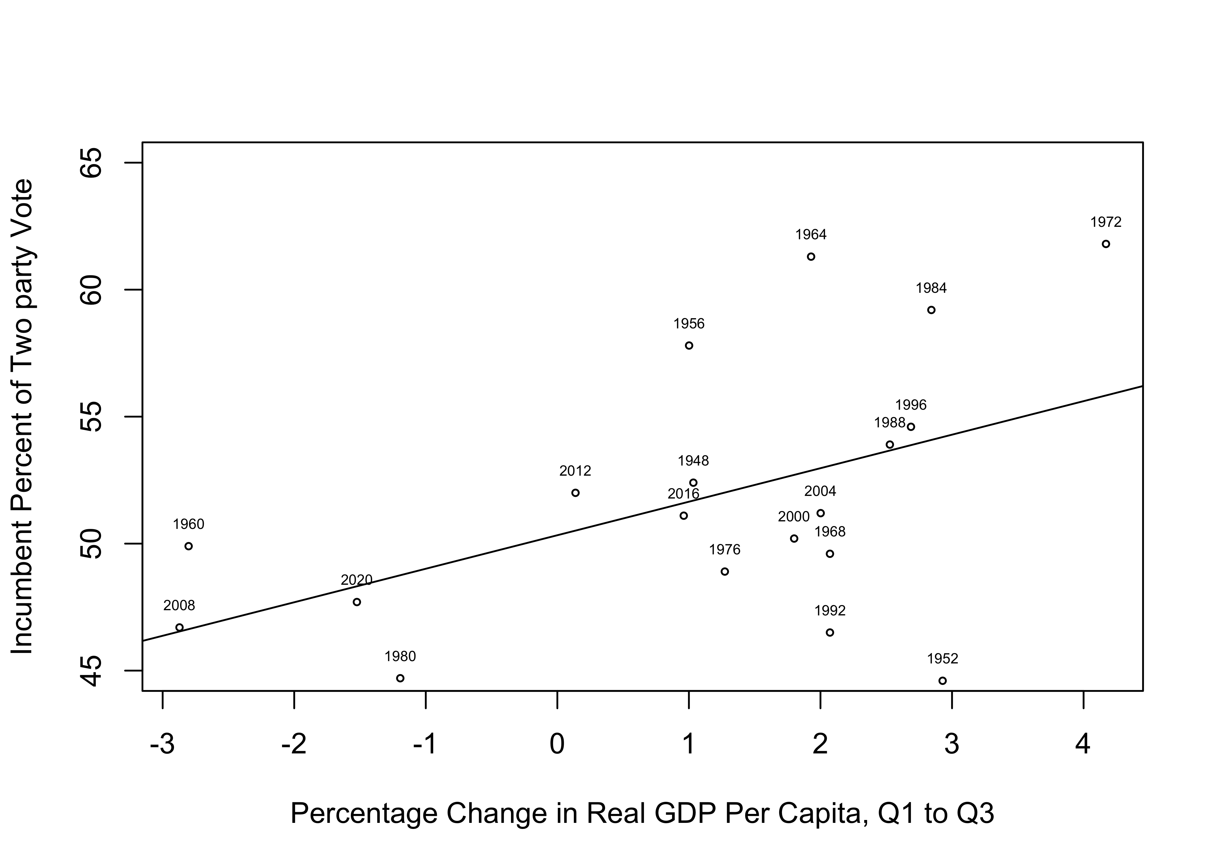
Figure 1.3: A Simple Test of the Retrospective Voting Hypothesis
Here is an example of the type of interpretation, based on these results, that makes it easier for the research consumer to understand the results of the analysis:
The results of the analysis provide some support for the retrospective voting hypothesis. The scatterplot shows that there is a general tendency for the incumbent party to struggle at the polls when the economy is relatively weak and to have success at the polls when the economy is strong. However, while there is a positive relationship between GDP growth and incumbent vote share, it is not a strong relationship. This can be seen in the variation in outcomes around the line of prediction, where we see a number of outcomes (1952, 1956, 1972, 1984, and 1992) that deviate quite a bit from the anticipated pattern. The correlation between these two variables (.49), confirms that there is a moderate, positive relationship between GDP growth and vote share for the incumbent presidential party. Clearly, there are other factors that help explain incumbent party electoral success, but this evidence shows that the state of the economy does play a role.
Feedback
Although it is generally accepted that theories should not be driven by what the data say (after all, the data are supposed to test the theory!), it would be foolish to ignore the results of the analysis and not allow for some feedback into the research process and reformulation of expectations. In other words, it is possible that you will discover something in the analysis that leads you to modify your theory, or at least change the way you think about things. In the real world of social science data analysis, there is a lot of back-and-forth between theory, hypothesis formation, and research findings. Typically, researchers have an idea of what they want to test, perhaps grounded in some form of theory, or maybe something closer to a solid rationale; they then gather data and conduct some analyses, sometimes finding interesting patterns that influence how they think about their research topic, even if they had not considered those things at the outset.
Let’s consider the somewhat modest relationship between change in GDP and votes for the incumbent party, as reported in Figure 1.3. Based on these findings, you could conclude that there is a tendency for the electorate to punish the incumbent party for economic downturns and reward it for economic upturns, but the trend is not strong. Alternatively, you could think about these results and ask ourselves if you are missing something. For instance, if the point of retrospective voting is to reward or punish the incumbent president for outcomes that occur during their presidency, then it should be easier to assign responsibility in years in which the president is running for another term. So, maybe we need to examine the two sets of elections (incumbent running vs. open seat) separately before concluding that the retrospective model is only somewhat supported by the data.
Figure 1.4 illustrates how important it can be to allow the results of the initial data analysis to provide feedback into the research process. On the left side, there is a fairly strong, positive relationship between changes in GDP in the first three quarters of the year and the incumbent party’s share of the two-party vote when the incumbent is running. There are a couple of years that deviate from the trend, but the overall pattern is much stronger here than it was in Figure 1.3, which included data from all elections. In addition, the scatterplot for open-seat contests (right side) shows that when the incumbent president is not running, there is virtually no relationship between the state of the economy and the incumbent party share of the two-party vote. These interpretations of the scatterplot patterns are further supported by the correlation coefficients, .68 for incumbent races and a meager .16 for open-seat contests.
[Figure******** 1.4 ********about here]
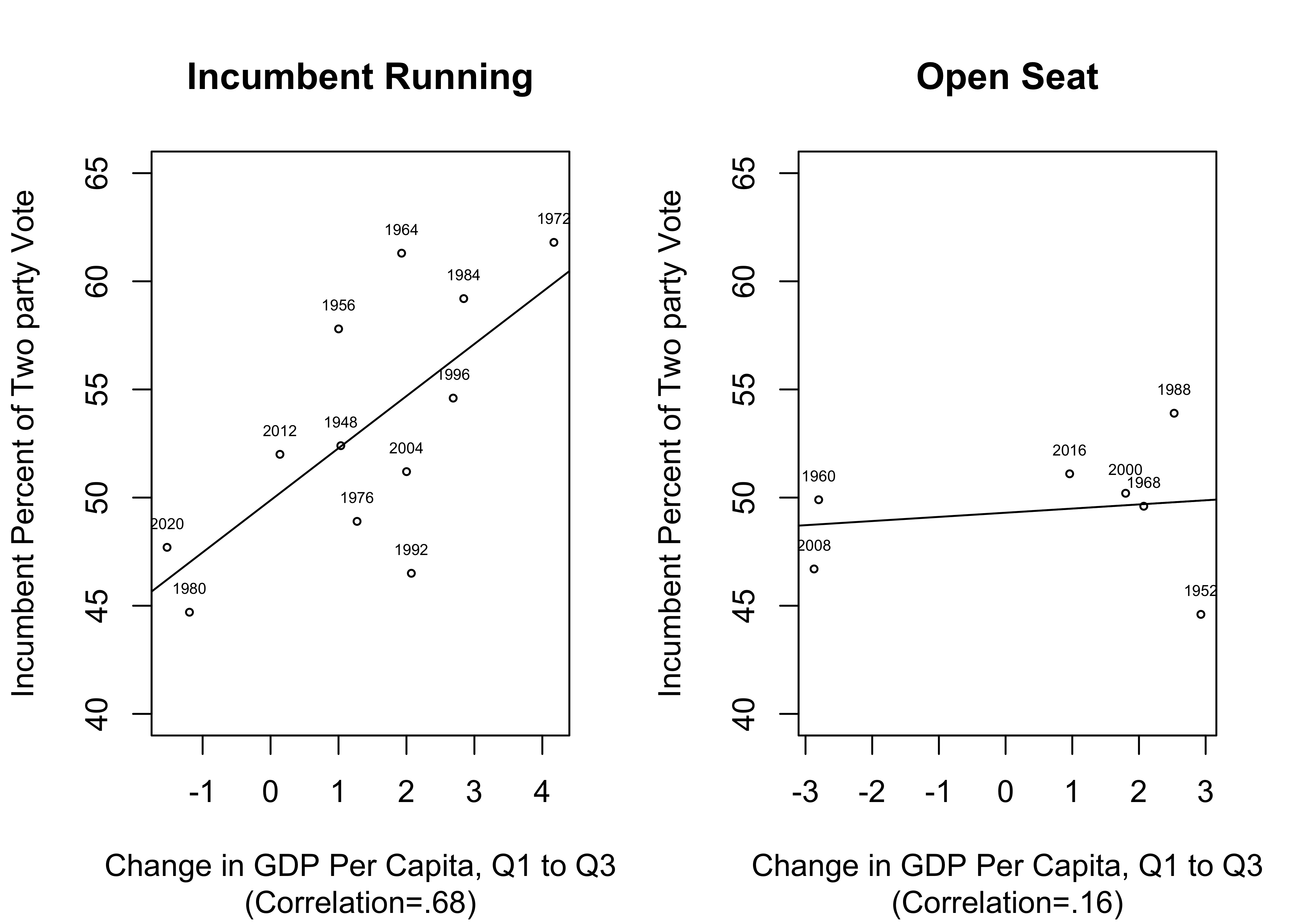
Figure 1.4: Testing the Retrospective Voting Hypothesis in Two Different Contexts
The lesson here is that it can be very useful to allow for some fluidity between the different components of the research process. When theoretically interesting possibilities present themselves during the data analysis stage, they should be given due consideration. Still, with this new found insight, it is necessary to exercise caution and not be over-confident in the results, in large part because they are based on only 19 elections. With such a small number of cases, the next two or three elections could alter the relationship in important ways if they do not fit the pattern of outcomes in Figure 1.4. This would not be as concerning if the findings were based on a larger sample of elections.
Causal Language
One important thing to remember when discussing linkages between variables is to be careful about the language you use to describe those relationships. You should understand the limits of what you can say regarding the causal mechanisms, while at the same time speaking confidently about what you think is going on in the data.
One way you can gain confidence in the causal nexus between variables, especially if you are using observational data, is by thinking about the necessary conditions for causality. By “necessary” conditions I mean those conditions that must be met if there is a causal relationship. These should not be taken as sufficient conditions, however. If one of the conditions is not met, then there is no causal relationship. If they are all met, then you are on surer footing but still don’t know that one variable “causes” the other. Meeting these conditions means that a causal relationship is possible.
Time order. Given our current understanding of how the universe operates, if X causes Y, then X must occur in time before Y.
Covariation. There must be an empirically discernible relationship between X and Y. If differences in X are not related to differences in Y, then it is hard to argue that outcomes on X play a role in shaping outcomes on Y.
Non-spurious. A spurious relationship between two variables is one that is produced by a third variable that is related to both the independent and dependent variables. In other words, while there may be a statistical relationship between X and Y, the relationship could reflect a third (confounding) variable that “causes” both X and Y. Remember, this is a problem with observational data but not experimental data. If you have heard researchers say something along the lines of “I have controlled for other influences,” that means they have tried to address this issue. This problem is covered more extensively in Chapters 14, 16, and 17).
Theoretical grounding. Are there strong theoretical reasons for believing that X causes Y? This takes us back to the earlier discussion of the importance of having clear expectations and a sound rationale for pursuing your line of research. This is important because variables are sometimes related to each other coincidentally and may satisfy the time-order criterion and the relationship may persist when controlling for other variables. But if the relationship is nonsensical, or at least seems like a real theoretical stretch, then it should not be assigned any causal significance.
Even if all of these conditions are met, it is important to remember that these are only necessary conditions. Satisfying these conditions is not a sufficient basis for making causal claims. Causal inferences must be made very cautiously, especially in a non-experimental setting.
Next Steps
This chapter reviewed a few of the topics and ideas that are important for understanding what data analysis is and what role it plays in the research process. Some of these things may still be hard for you to relate to at this point, especially if you have not been involved in a quantitative research project. Much of what is covered here will come up again in subsequent parts of the book, hopefully solidifying your grasp of the material.
The next couple of chapters cover other foundational material. Chapter 2 focuses on how to access R and use it for some simple tasks, such as examining imported data sets, and Chapter 3 introduces you to some basic statistical tables and graphs. As you read these chapters, it is very important that you follow the R demonstrations closely. In fact, I encourage you to make sure you can access R (download it or, preferably, use RStudio via Posit.cloud) and follow along, running the same R code you see in the book, so you don’t have to wait for an assignment to get your first hands on experience.
A quick word of warning, there will be errors. You should reconcile yourself now to getting errors while working in R, especially in the first few chapters. In fact, I made several errors trying to get things to run correctly so I could present the results you will see the next couple of chapters. The great thing about this is that I learned a little bit from every error I made. You will have a much better experience if you can learn to chill about error messages. Between this book and help from your instructor, you will figure it out. Forge ahead, make mistakes, and learn!
Exercises
Concepts and Calculations
Identify the level of measurement (nominal, ordinal, interval/ratio) and divisibility (discrete or continuous) for each of the following variables.
- Course letter grade
- Voter turnout rate (%)
- Marital status (Married, divorced, single, etc)
- Occupation (Professor, cook, mechanic, etc.)
- Body weight
- Total number of votes cast
- #Years of education
- Subjective social class (Poor, working class, middle class, etc.)
- % below poverty level income
- Racial or ethnic group identification
For each of the pairs of variables listed below, designate which one you think should be the dependent variable and which is the independent variable. Give a brief explanation.
- Poverty rate/Voter turnout
- Annual Income/Years of education
- Racial group/Vote choice
- Study habits/Course grade
- Average Life expectancy/Gross Domestic Product
- Social class/happiness
Assume that the topics listed below represent different research topics and classify each of them each of them as either a “political” or “social” topic. Justify your classification. If you think a topic could be classified either way, explain why.
- Marital Satisfaction
- Racial inequality
- Campaign spending
- Welfare policy
- Democratization
- Attitudes toward abortion
- Teen pregnancy
For each of the pairs of terms listed below, identify which one represents a concept, and which one is an operational variable.
- Political participation/Voter turnout
- Annual income/Wealth
- Restrictive COVID-19 Rules/Mandatory masking policy
- Economic development/Per capita GDP
What is a broad social or political subject area that interests you? Within that area, what is a narrower topic of interest? Given that topic of interest, what is a research question you think would be interesting to pursuing? Finally, share a hypothesis related to the research question that you think would be interesting to test.
A researcher asked people taking a survey if they were generally happy or unhappy with the way life was going for them. They repeated this question in a followup survey two weeks later and found that 85% of respondents provided the same response. Is this a demonstration of validity or reliability? Why?
In an introductory political science class, there is a very strong relationship between accessing online course materials and course grade at the end of the semester: Generally, students who access course material frequently tend to do well, while those who don’t access course material regularly tend to do poorly. This leads to the conclusion that accessing course material has a causal impact on course performance. What do you think? Does this relationship satisfy the necessary conditions for establishing causality? Address this question using all four conditions.
A scholar is interested in examining the impact of electoral systems on levels of voter turnout using data from a sample of 75 countries. The primary hypothesis is that voter turnout (% of eligible voters who vote) is higher in electoral systems that use proportional representation than in majoritarian/plurality systems.
- Is this an experimental study or an an observational study?
- What is the dependent variable, and what is its level of measurement?
- What is the independent variable, and what is its level of measurement?
- What is the level of analysis for this study?