Multivariate Statistical Analysis using R
2019-12-16
Chapter 1 Principal Component Analysis
Advice: Use the simplest method that provides the clearest picture.
Principal component analysis (PCA) is used to analyze one table of quantitative data. PCA mixes the input variables to give new variables, called principal components. The first principal component is the line of best fit. It is the line that maximizes the inertia (similar to variance) of the cloud of data points. Subsequent components are defined as orthogonal to previous components, and maximize the remaining inertia.
PCA gives one map for the rows (called factor scores), and one map for the columns (called loadings). These 2 maps are related, because they both are described by the same components. However, these 2 maps project different kinds of information onto the components, and so they are interpreted differently. Factor scores are the coordinates of the row observations. They are interpreted by the distances between them, and their distance from the origin. Loadings describe the column variables. Loadings are interpreted by the angle between them, and their distance from the origin.
The distance from the origin is important in both maps, because squared distance from the mean is inertia (variance, information; see sum of squares as in ANOVA/regression). Because of the Pythagorean Theorem, the total information contributed by a data point (its squared distance to the origin) is also equal to the sum of its squared factor scores.
1.0.1 PCA Data: PHQ
The Patient Health Questionnaire is a survey that is a preliminary measurement for depression severity.
There are 9 questions (columns) measured on a scale from 1 i.e. “no days” to 4 “nearly every day” and 225 participants (rows).
The descriptors of the pariticpants are memory group, sex, and age. For this analysis I will be using memory group that is either high, normal, or low memory.
| Pleasure | Hopeless | Sleep | Energy | Appetite | Failure | Focus | Speed | Suicide |
|---|---|---|---|---|---|---|---|---|
| 1 | 1 | 2 | 3 | 1 | 1 | 1 | 1 | 1 |
| 1 | 1 | 1 | 2 | 1 | 1 | 1 | 1 | 1 |
| 1 | 1 | 1 | 1 | 1 | 1 | 1 | 1 | 1 |
| 1 | 3 | 4 | 2 | 3 | 2 | 1 | 1 | 1 |
| 1 | 1 | 1 | 1 | 1 | 1 | 1 | 1 | 1 |
| 1 | 2 | 3 | 3 | 1 | 3 | 2 | 1 | 1 |
1.1 PCA correlation plot
cor.res <- cor(PHQ)
corrplot.mixed(cor.res, tl.cex = 0.7, tl.col = "black", addCoefasPercent = TRUE)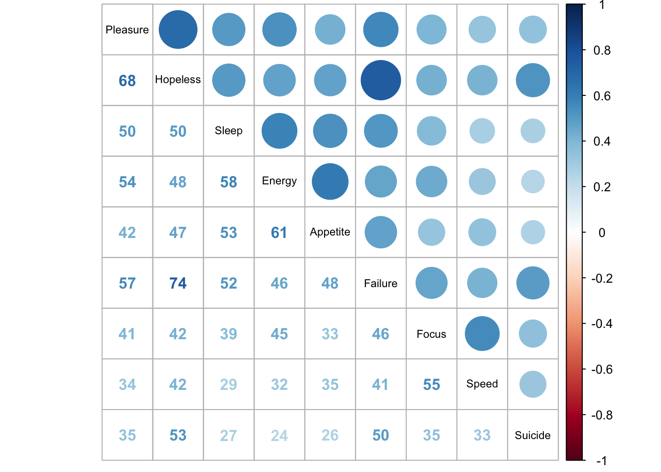
#cor.plot <- recordPlot() # you need this line to be able to save the figure to PPT later
memory <- matrix(,nrow = nrow(PHQ), ncol = 1)
memory[1:72] <- 3 #high memory
memory[73:144] <-2 #norm memory
memory[145:216] <-1 #low memory

#Totalscore and Memory design variables correlation
TotalscoreMemory <- cbind(data.frame(totalscore), data.frame(memory))
colnames(TotalscoreMemory) <- c("Totalscore","Memory")

PHQ9BeckScatter <- ggscatter(TotalscoreMemory, x = "Totalscore", y = "Memory",
          add = "reg.line", conf.int = TRUE, color = 'mediumorchid4',
          cor.coef = TRUE, cor.method = "pearson",
          xlab = "Depression Severity", ylab = "Memory Group")
PHQ9BeckScatter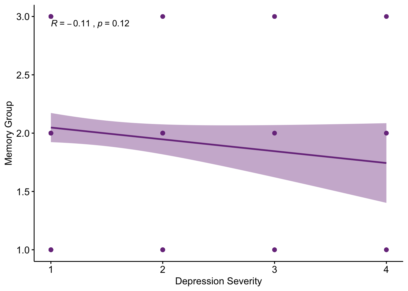
We can see that all questions are positively correlated with each other. Feelings of failure and hopleness have the highest correlation of .74. Loss of pleasure and hopeless are also highly correlated (.68).
From the correlation plot we can see that in this data set depression severity is not significantly correlated with what memory group the participants are in.
1.2 PCA Analysis
## [1] "It is estimated that your iterations will take 0.01 minutes."
## [1] "R is not in interactive() mode. Resample-based tests will be conducted. Please take note of the progress bar."
## ===========================================================================
1.2.1 PCA Testing the eigenvalues
zeDim = 1
pH1 <- prettyHist(
  distribution = res_pcaInf$Inference.Data$components$eigs.perm[,zeDim],
           observed = res_pcaInf$Fixed.Data$ExPosition.Data$eigs[zeDim],
           xlim = c(200, 1300), # needs to be set by hand
           breaks = 20,
           border = "white",
           main = paste0("Permutation Test for Eigenvalue ",zeDim),
           xlab = paste0("Eigenvalue ",zeDim),
           ylab = "",
           counts = FALSE,
           cutoffs = c( 0.975))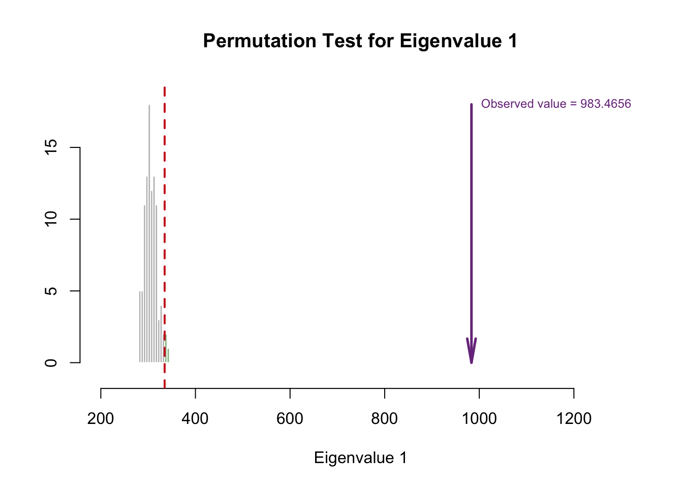
#eigs1 <- recordPlot()
zeDim = 2
pH2 <- pH1 <- prettyHist(
  distribution = res_pcaInf$Inference.Data$components$eigs.perm[,zeDim],
           observed = res_pcaInf$Fixed.Data$ExPosition.Data$eigs[zeDim],
           xlim = c(200, 350), # needs to be set by hand
           breaks = 20,
           border = "white",
           main = paste0("Permutation Test for Eigenvalue ",zeDim),
           xlab = paste0("Eigenvalue ",zeDim),
           ylab = "",
           counts = FALSE,
           cutoffs = c(0.975))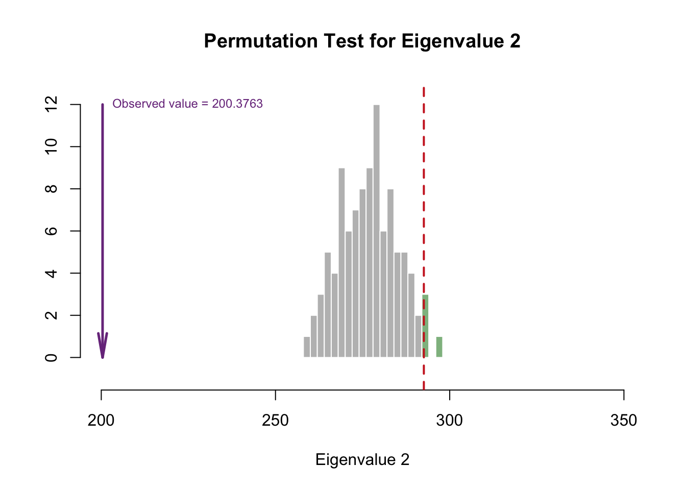
Eigenvalue 1 is reliable, but eigenvalue 2 doesn’t look reliable. However, that doesn’t mean we ignore the second eigenvalue!!
1.2.2 PCA Scree Plot
my.scree <- PlotScree(ev = res_pcaInf$Fixed.Data$ExPosition.Data$eigs,
                      p.ev = res_pcaInf$Inference.Data$components$p.vals, plotKaiser = TRUE)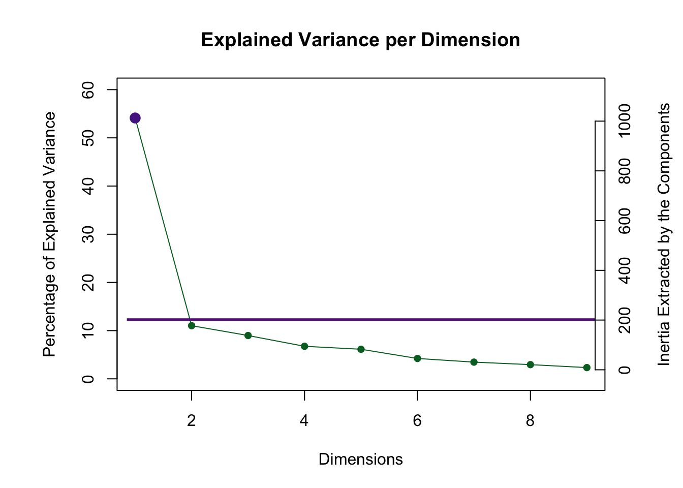
Dimension 1 is abvoe the Kaiser cut off and dimension 2 is really close!
1.2.3 PCA Factor scores
my.fi.plot <- createFactorMap(res_pcaInf$Fixed.Data$ExPosition.Data$fi, # data
                            title = "PHQ Row Factor Scores", # title of the plot
                            axis1 = 1, axis2 = 2, # which component for x and y axes
                            pch = 19, # the shape of the dots (google `pch`)
                            cex = 2, # the size of the dots
                            display.labels = FALSE,
                            text.cex = 2.5, # the size of the text
                            alpha.points = 0.3,
                            col.points = res_pcaInf$Fixed.Data$Plotting.Data$fi.col, # color of the dots
                            col.labels = res_pcaInf$Fixed.Data$Plotting.Data$fi.col, # color for labels of dots
                            )

fi.labels <- createxyLabels.gen(1,2,
                             lambda = res_pcaInf$Fixed.Data$ExPosition.Data$eigs,
                             tau = round(res_pcaInf$Fixed.Data$ExPosition.Data$t),
                             axisName = "Component "
                             )
fi.plot <- my.fi.plot$zeMap + fi.labels # you need this line to be able to save them in the end
fi.plot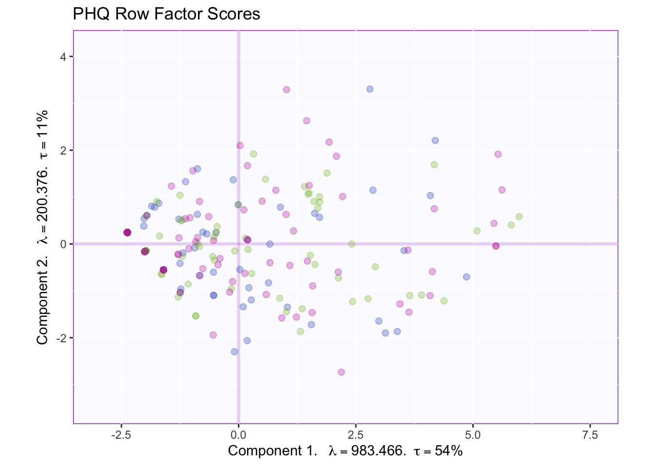
As the rows move from left to right the variance starts smaller and then gradually increases and slighlty decreases again. However, from this plot it is hard to tell what is happening on each component.
1.2.3.1 PCA With group means
#Get color for each group
# get index for the first row of each group
grp.ind <- order(GroupingVaribles$memoryGroups)[!duplicated(sort(GroupingVaribles$memoryGroups))]
grp.col <- res_pcaInf$Fixed.Data$Plotting.Data$fi.col[grp.ind] # get the color
grp.name <- GroupingVaribles$memoryGroups[grp.ind] # get the corresponding groups
names(grp.col) <- grp.name

#Get means
group.mean <- aggregate(res_pcaInf$Fixed.Data$ExPosition.Data$fi,
                     by = list(GroupingVaribles$memoryGroups), # must be a list
                     mean)

# need to format the results from `aggregate` correctly
rownames(group.mean) <- group.mean[,1] # Use the first column as row names
fi.mean <- group.mean[,-1] # Exclude the first column

#Plot it!
fi.mean.plot <- createFactorMap(fi.mean,
                                alpha.points = 0.8,
                                col.points = grp.col[rownames(fi.mean)],
                                col.labels = grp.col[rownames(fi.mean)],
                                pch = 17,
                                cex = 3,
                                text.cex = 3)
fi.WithMean <- my.fi.plot$zeMap_background + my.fi.plot$zeMap_dots + fi.mean.plot$zeMap_dots + fi.mean.plot$zeMap_text + fi.labels
fi.WithMean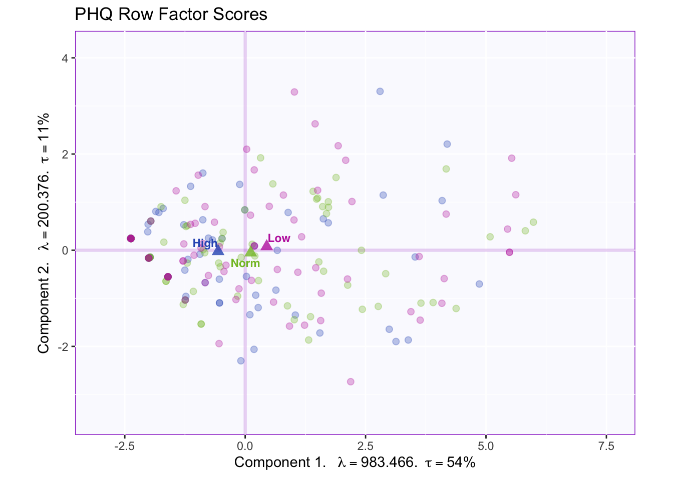
All the group means fall on or very close to component 1.
1.2.4 PCA Tolerance interval
We can plot the tolerance interval
TIplot <- MakeToleranceIntervals(res_pcaInf$Fixed.Data$ExPosition.Data$fi,
                            design = as.factor(GroupingVaribles$memoryGroups),
                            # line below is needed
                            names.of.factors =  c("Dim1","Dim2"), # needed
                            col = grp.col[rownames(fi.mean)],
                            line.size = .50,
                            line.type = 3,
                            alpha.ellipse = .2,
                            alpha.line    = .4,
                            p.level       = .95)

fi.WithMeanTI <- my.fi.plot$zeMap_background + my.fi.plot$zeMap_dots + fi.mean.plot$zeMap_dots + fi.mean.plot$zeMap_text + TIplot + fi.labels

fi.WithMeanTI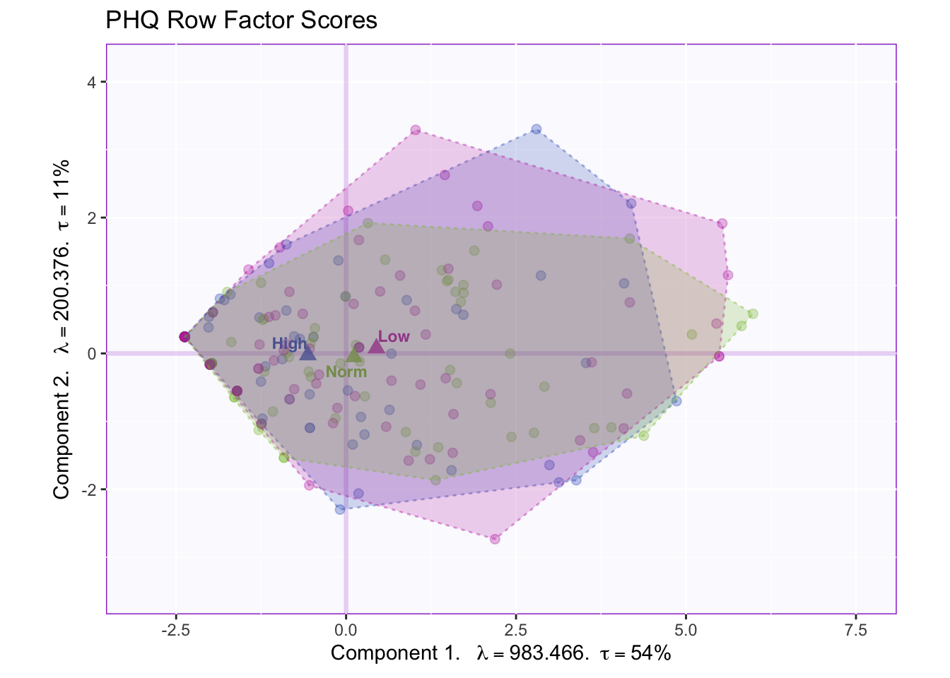
The tolerance interval shows there is overlap of the distribution of the data points in the groups.
1.2.5 PCA Bootstrap interval
#We can also add the bootstrap interval for the group means to see if these group means are significantly different.

#First step: bootstrap the group means

# Depend on the size of your data, this might take a while
fi.boot <- Boot4Mean(res_pcaInf$Fixed.Data$ExPosition.Data$fi,
                     design = GroupingVaribles$memoryGroups,
                     niter = 1000)

# Check other parameters you can change for this function
bootCI4mean <- MakeCIEllipses(fi.boot$BootCube[,c(1:2),], # get the first two components
                              col = grp.col[rownames(fi.mean)])

fi.WithMeanCI <- my.fi.plot$zeMap_background + bootCI4mean + my.fi.plot$zeMap_dots + fi.mean.plot$zeMap_dots + fi.mean.plot$zeMap_text + fi.labels
fi.WithMeanCI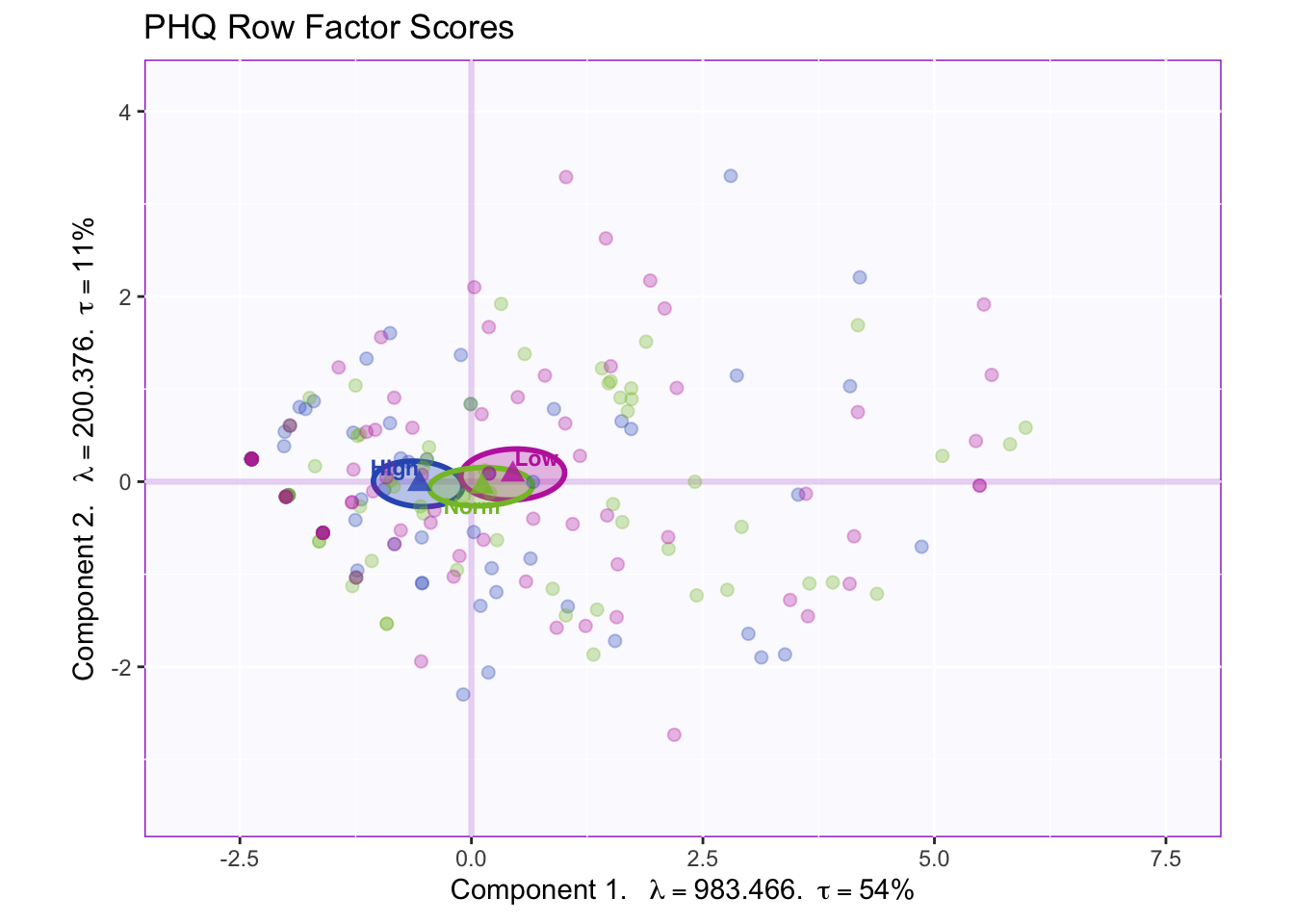
With a smaller sample size, we can conclude that the groups are not reliably different from one another due to all confidence intervals overlapping.
1.2.6 PCA Loadings
colnames(res_pcaInf$Fixed.Data$ExPosition.Data$fi) <- c('Pleasure','Hopeless','Sleep','Energy','Appetite','Failure','Focus','Speed','Suicide')
cor.loading <- cor(PHQ, res_pcaInf$Fixed.Data$ExPosition.Data$fi)
rownames(cor.loading) <- colnames(cor.loading)

#Get colors for different variables
VariableColors <- prettyGraphsColorSelection(n.colors = ncol(PHQ))

loading.plot <- createFactorMap(cor.loading,
                                constraints = list(minx = -1, miny = -1,
                                                   maxx = 1, maxy = 1),
                                col.points = VariableColors,
                                col.labels = VariableColors)
LoadingMapWithCircles <- loading.plot$zeMap +
  addArrows(cor.loading, color = VariableColors) +
  addCircleOfCor() + xlab("Component 1") + ylab("Component 2")

LoadingMapWithCircles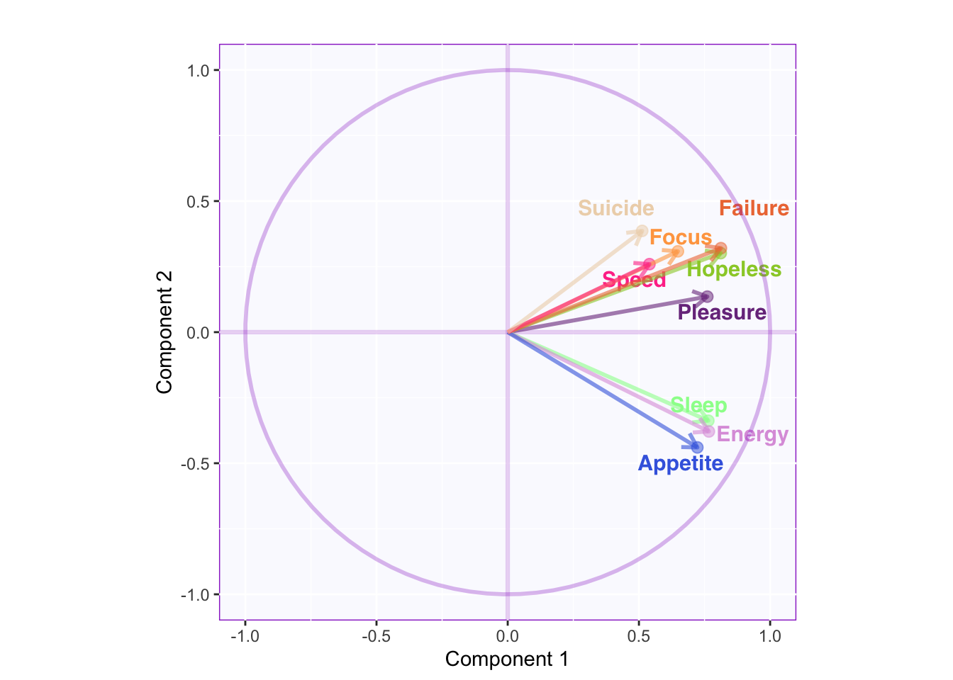
Component 1: All variables are positively correlated.
Component 2: Sleep, Energy, and Appetite seem to be less correlated to the rest of the variables (approaching orthogonality).
More of the variance for Suicide, Speed, and Focus seem to be in a different dimension.
#You can also include the variance of each component and plot the factor scores for the columns (i.e., the variables):
my.fj.plot <- createFactorMap(res_pcaInf$Fixed.Data$ExPosition.Data$fj, # data
                            title = "PHQ Column Loadings", # title of the plot
                            axis1 = 1, axis2 = 2, # which component for x and y axes
                            pch = 19, # the shape of the dots (google `pch`)
                            cex = 3, # the size of the dots
                            text.cex = 3, # the size of the text
                            col.points = VariableColors, # color of the dots
                            col.labels = VariableColors, # color for labels of dots
                            )

fj.plot <- my.fj.plot$zeMap + fi.labels # you need this line to be able to save them in the end
fj.plot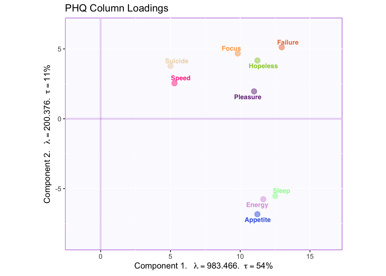
Component 1: All Symptoms
Component 2: Emotional symptoms vs physical symptoms
1.2.6.1 PCA Bootstrap Ratio of columns
_**Note: This is not the same as the contribution bars_
1.2.6.1.1 PCA Component 1 and 2
signed.ctrJ <- res_pcaInf$Fixed.Data$ExPosition.Data$cj * sign(res_pcaInf$Fixed.Data$ExPosition.Data$fj)

# plot contributions for component 1
ctrJ.1 <- PrettyBarPlot2(signed.ctrJ[,1],
                         threshold = 1 / NROW(signed.ctrJ),
                         font.size = 5,
                         color4bar = gplots::col2hex(VariableColors), # we need hex code
                         ylab = 'Contributions',
                         ylim = c(1.2*min(signed.ctrJ), 1.2*max(signed.ctrJ))
) + ggtitle("Contribution barplots", subtitle = 'Component 1: Variable Contributions (Signed)')

# plot contributions for component 2
ctrJ.2 <- PrettyBarPlot2(signed.ctrJ[,2],
                         threshold = 1 / NROW(signed.ctrJ),
                         font.size = 5,
                         color4bar = gplots::col2hex(VariableColors), # we need hex code
                         ylab = 'Contributions',
                         ylim = c(1.2*min(signed.ctrJ), 1.2*max(signed.ctrJ))
) + ggtitle("",subtitle = 'Component 2: Variable Contributions (Signed)')


BR <- res_pcaInf$Inference.Data$fj.boots$tests$boot.ratios
laDim = 1

# Plot the bootstrap ratios for Dimension 1
ba001.BR1 <- PrettyBarPlot2(BR[,laDim],
                        threshold = 2,
                        font.size = 5,
                   color4bar = gplots::col2hex(VariableColors), # we need hex code
                  ylab = 'Bootstrap ratios'
                  #ylim = c(1.2*min(BR[,laDim]), 1.2*max(BR[,laDim]))
) + ggtitle("Bootstrap ratios", subtitle = paste0('Component ', laDim))

# Plot the bootstrap ratios for Dimension 2
laDim = 2
ba002.BR2 <- PrettyBarPlot2(BR[,laDim],
                        threshold = 2,
                        font.size = 5,
                   color4bar = gplots::col2hex(VariableColors), # we need hex code
                  ylab = 'Bootstrap ratios'
                  #ylim = c(1.2*min(BR[,laDim]), 1.2*max(BR[,laDim]))
) + ggtitle("",subtitle = paste0('Component ', laDim))
#We then use the next line of code to put two figures side to side:
grid.arrange(
as.grob(ctrJ.1),
as.grob(ctrJ.2),
as.grob(ba001.BR1),
as.grob(ba002.BR2),
ncol = 2,nrow = 2,
top = textGrob("Barplots for variables", gp = gpar(fontsize = 18, font = 3))
)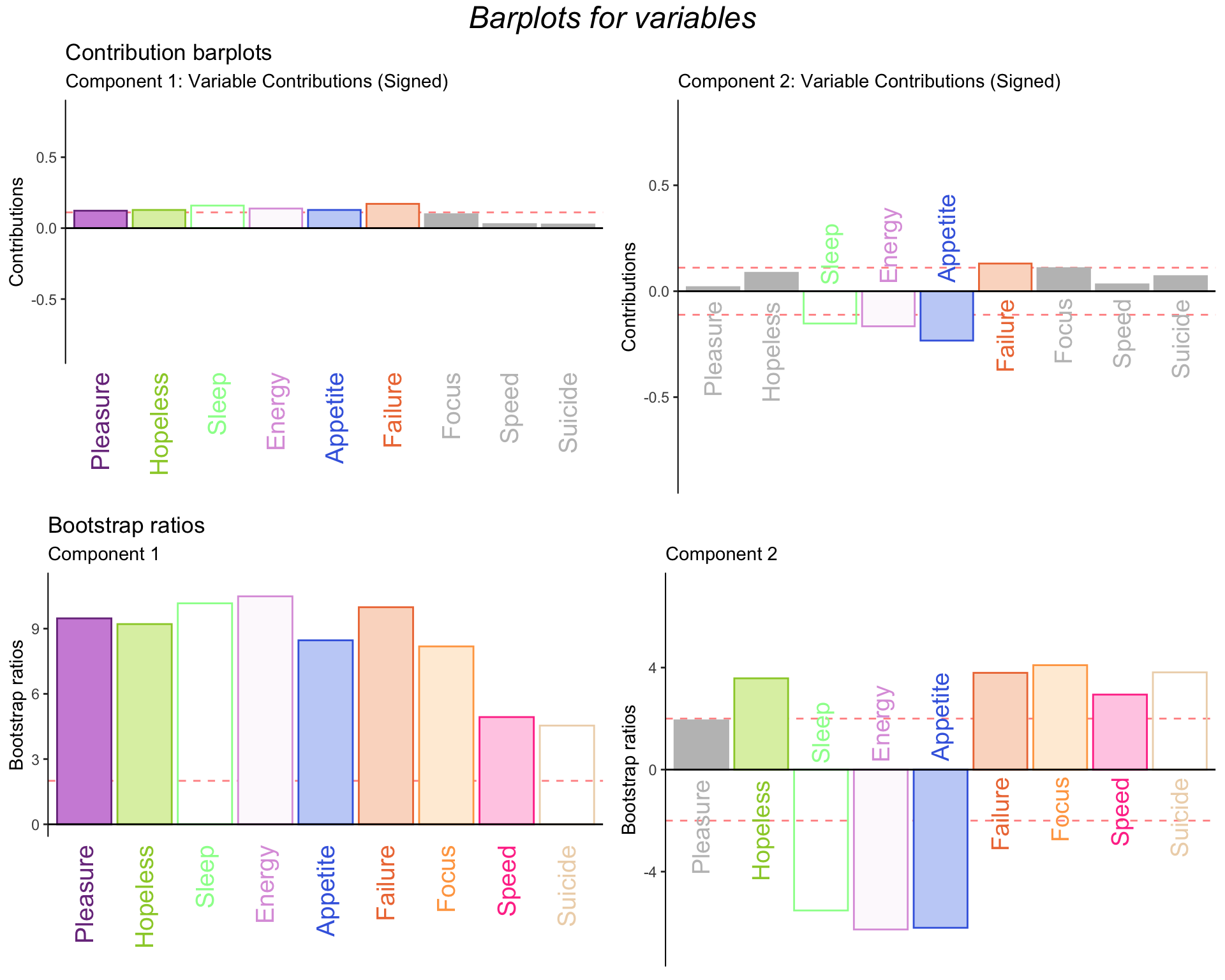
Component 1: The variables with the greatest contributions are all but Focus, Speed, and Suicide.
Component 2: Failure is positively contributing while Sleep, Energy, and Appetite are negatively contributing.
The barplots for bootstrap ratios show that all the variables that contributed a signficant amount are actually significant.
1.3 Summary
When we interpret the factor scores and loadings together, the PCA revealed:
Component 1: Regardless of memory group they all experience more of the symptoms, except feelings of suicide, loss of focus, and distrubances in speed i.e. feeling hyperactive or lethargic.
Component 2: All memory groups experience more appetite, sleep, and energy when they have only increased feelings of faliure.
Both: When all memory groups experience increases in only one symptom they experience the other symptoms differently than compared to when they experience increases in all symptoms together.