Chapter 3 Correspondence Analysis

PCA for two qualitative variables represented by a contingency table. The data set has variables in the rows AND columns and each element of the contingency table is the number of observations.

The barycenter is found by multiplying the inverse of the total of the contingency table by the total of the columns:

                    ((1xI)(IxJ)(Jx1))^-1 * (1xI)(IxJ)

The contingency table is transformed into a probability matrix by multiplying the rows by their masses and the columns by their weight. The masses are obtained by the inverse of the total of the contingency table multiplied by the total of the rows:

                   M = diag((1xI)(IxJ)(Jx1))^-1 * (IxJ)(Jx1)

The weights are obtained by the inverse of the columns componenet to the barycenter: W = diag(((1xI)(IxJ)(Jx1))^-1 * (1xI)(IxJ))^-1

Finally, GSVD is applied to the new probability matrix with the constraints:

                    t(P)MP = t(Q)WQ = I

3.1 Data set: Beer

It is a contingency table of 9 different beers (rows) on 30 beer characteristics (columns).

	bitter	complement	goodcolor	picon	good	pot	clear	disappointing	refreshing	golden	queasy	aperitif	bland	floral
Alken	3	5	21	3	17	3	26	9	15	17	2	8	20	3
Bavik	2	5	19	3	21	7	18	7	17	17	5	8	6	13
Bock	5	4	9	1	11	1	33	18	11	10	9	3	8	3
Emelisse	50	2	15	5	3	6	2	25	2	15	17	4	7	3
Jupiler	6	2	8	4	12	1	34	18	18	13	1	2	26	4
Moor	41	3	6	1	2	3	16	21	8	6	26	4	6	5
Piedboeuf	1	7	26	1	12	3	1	14	11	28	2	1	23	4
Ridder	20	3	5	6	6	3	16	17	7	6	20	1	14	3
Simcoe	36	3	17	1	9	4	3	15	6	13	14	5	7	3

3.2 The Data Pattern

# get Chi2 -- we can use the available package to get the Chi2
suppressWarnings(chi2    <-  chisq.test(Beer))

# Components of chi2: the chi-squares for each cell before we add them up to compute the chi2
Inertia.cells <- chi2$residuals / sqrt(sum(Beer))
# To be Plotted

corrplot(Inertia.cells, is.cor = FALSE, tl.cex = .7, method = "color")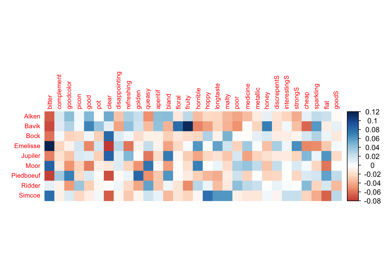

#a0.residuals <- recordPlot()

From the correlation plot it seems bitterness has the strongest correlation with all the beers except Ridder.

3.3 Analysis

3.3.1 Symmetric

# run CA
resCA.sym  <- epCA(Beer, DESIGN = BeerGrouped$GroupBeer, make_design_nominal = TRUE, symmetric = TRUE, graphs = FALSE)

# Rows
resCAinf.sym4bootJ  <- epCA.inference.battery(Beer, DESIGN = BeerGrouped$GroupBeer, make_design_nominal = TRUE, symmetric = TRUE, graphs = FALSE)

## [1] "It is estimated that your iterations will take 0.02 minutes."
## [1] "R is not in interactive() mode. Resample-based tests will be conducted. Please take note of the progress bar."
## ===========================================================================

# Columns
resCAinf.sym4bootI  <- epCA.inference.battery(t(Beer), DESIGN = BeerGrouped$GroupBeer, make_design_nominal = TRUE, symmetric = TRUE, graphs = FALSE)

## [1] "Row dimensions do not match for X and Y. Creating default."
## [1] "It is estimated that your iterations will take 0.02 minutes."
## [1] "R is not in interactive() mode. Resample-based tests will be conducted. Please take note of the progress bar."
## ===========================================================================

3.3.2 Asymmetric

# to run a plain CA but asymmetric
# this is using the columns as the simplex (you can also use rows by running epCA with t(X))
resCA.asym <- epCA(Beer, DESIGN = BeerGrouped$GroupBeer, make_design_nominal = TRUE, symmetric = FALSE, graphs = FALSE)

3.3.3 Scree Plot

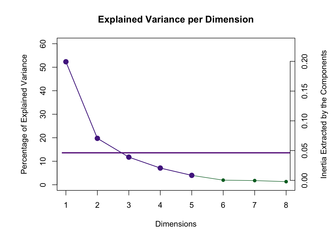
Even though 5 dimensions are reliable via the permutation test only 2 are above the Kaiser line.

3.3.4 Plot the Asymmetric Factor scores

#Makes legend for Expert Groups
plot(NULL, xaxt = 'n', yaxt = 'n', bty = 'n', ylab = '', xlab = '', xlim = 0:1, ylim = 0:1)
legend("topleft", legend=c("Sweet", "Bland", "Hoppy"),
      col=c("#305ABF", "#84BF30", "#BF30AD"),pch = 16, pt.cex = 2, cex=0.75, bty = 'n')
mtext("Expert Rating", at = 0.1, cex = 1.5)

3.3.5 Asymmetric Map

# Here are the factor scores you need
Fj.a <- resCA.asym$ExPosition.Data$fj
Fi   <- resCA.sym$ExPosition.Data$fi
Fj   <- resCA.sym$ExPosition.Data$fj

# constraints -----
# first get the constraints correct
constraints.sym  <- minmaxHelper(mat1 = Fi, mat2  = Fj)
constraints.asym <- minmaxHelper(mat1 = Fi, mat2  = Fj.a)

# Get some colors ----
color4Beers <-prettyGraphsColorSelection(n.colors = nrow(Fi))
# baseMaps ----
colnames(Fi) <- paste("Dimension ", 1:ncol(Fi))
colnames(Fj) <- paste("Dimension ", 1:ncol(Fj))
colnames(Fj.a) <- paste("Dimension ", 1:ncol(Fj.a))

# Your asymmetric factor scores
asymMap  <- createFactorMapIJ(Fi,Fj.a,
                              col.points.i = gplots::col2hex(resCA.sym$Plotting.Data$fi.col),
                              col.labels.i = gplots::col2hex(resCA.sym$Plotting.Data$fi.col))

# Make the simplex visible
polygonorder <- c(1, 18, 6, 15, 5, 28, 29, 7, 27, 20, 16)
zePoly.J <-  PTCA4CATA::ggdrawPolygon(Fj.a, order2draw = polygonorder, 
                                      color = 'darkolivegreen4',
                                      size = .2, 
                                      fill =  'darkolivegreen4',
                                      alpha = .1)
# Labels
labels4CA <- createxyLabels(resCA = resCA.asym)

# Combine all elements you want to include in this plot
map.I.asym <- asymMap$baseMap + zePoly.J + 
                          asymMap$I_points +
                          asymMap$J_labels + asymMap$J_points +
                          labels4CA + 
ggtitle('Asymmetric Map Simplex') 
map.I.asym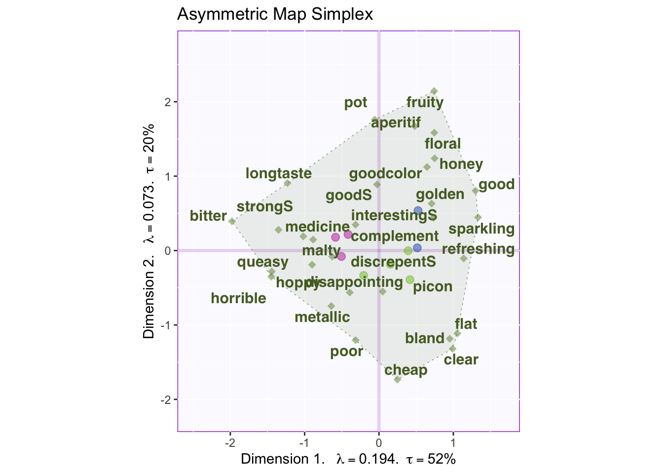

Asymmetric uses the columns (weights) as the axis for the simplex and the rows (masses) are typically contained within. In asymmetric we can interpret the rows and columns together.

3.3.6 Symmetric Map

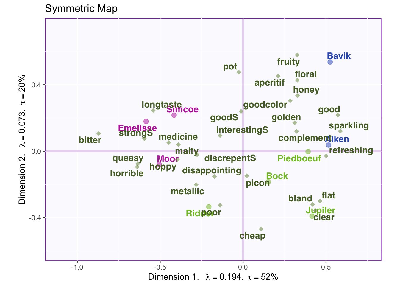
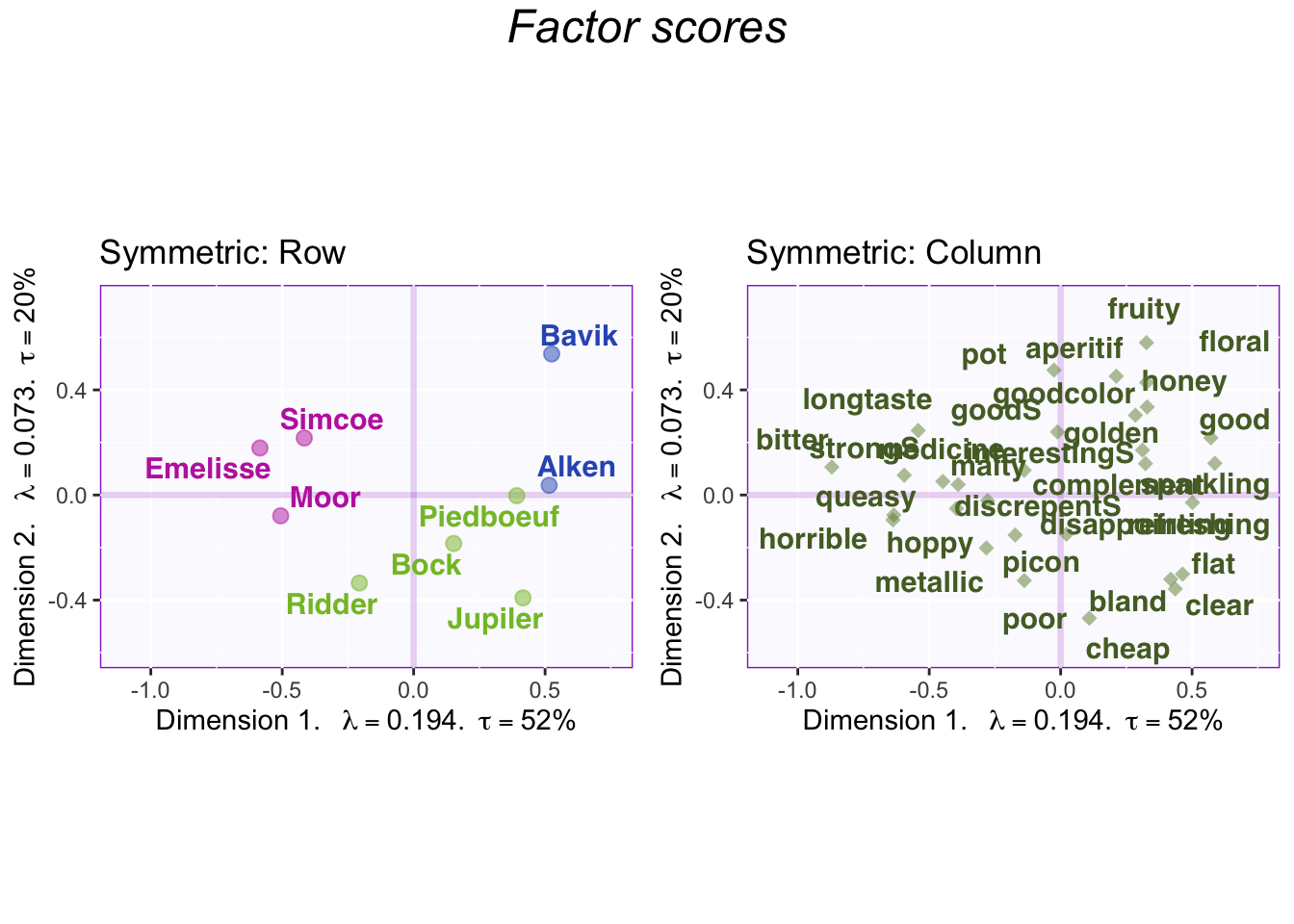
Symmetric plots normalize the rows and the columns differently. Therefore, we can only compare rows to rows and columns to columns. When interpreting the columns and rows together it needs to be interpreted against the mean (origin) instead of each other.

3.3.7 Factor Scores with Symmetric Map

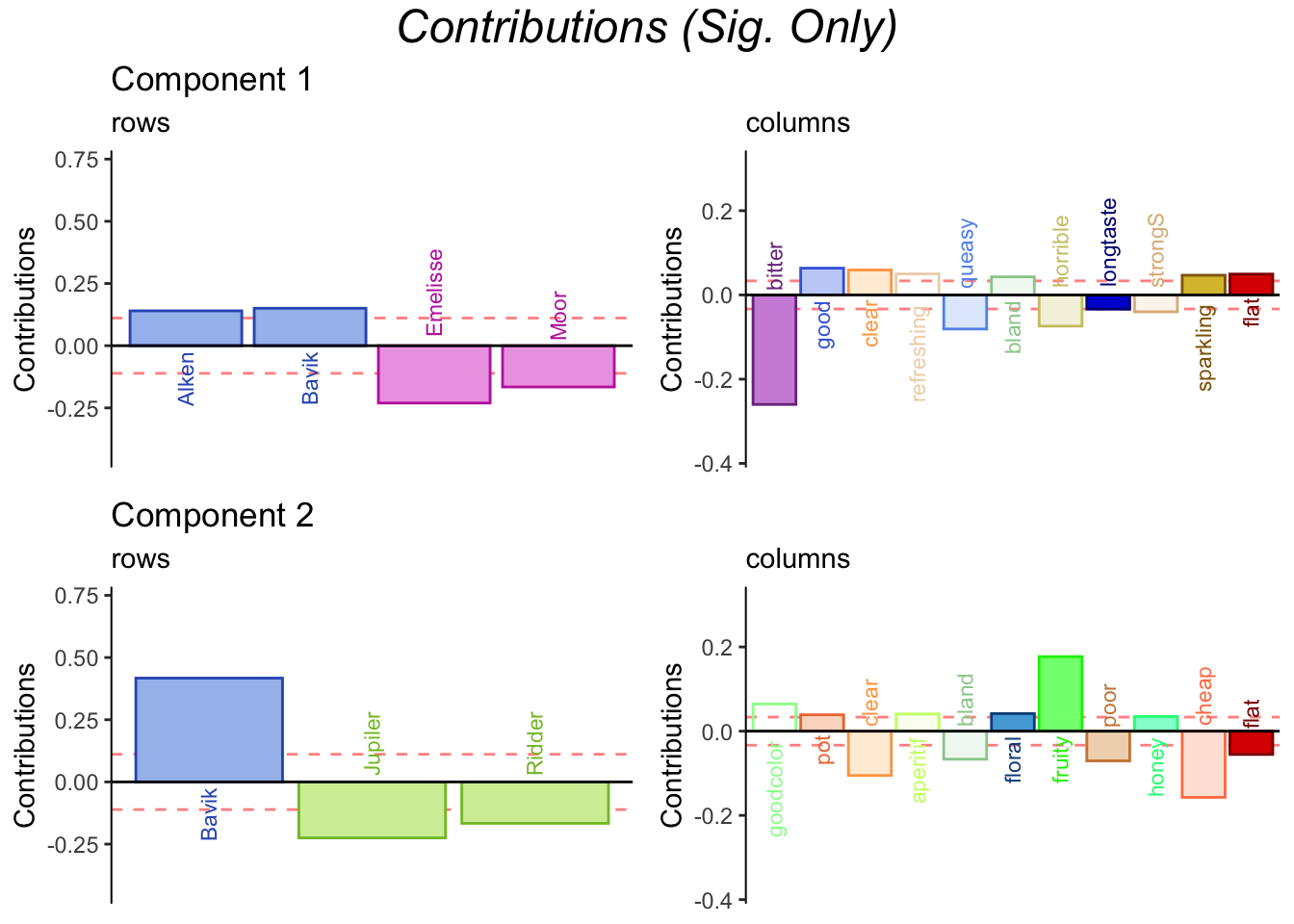
3.3.8 Contributions and bootstrap ratios barplots

3.3.9 Bootstrap Ratios

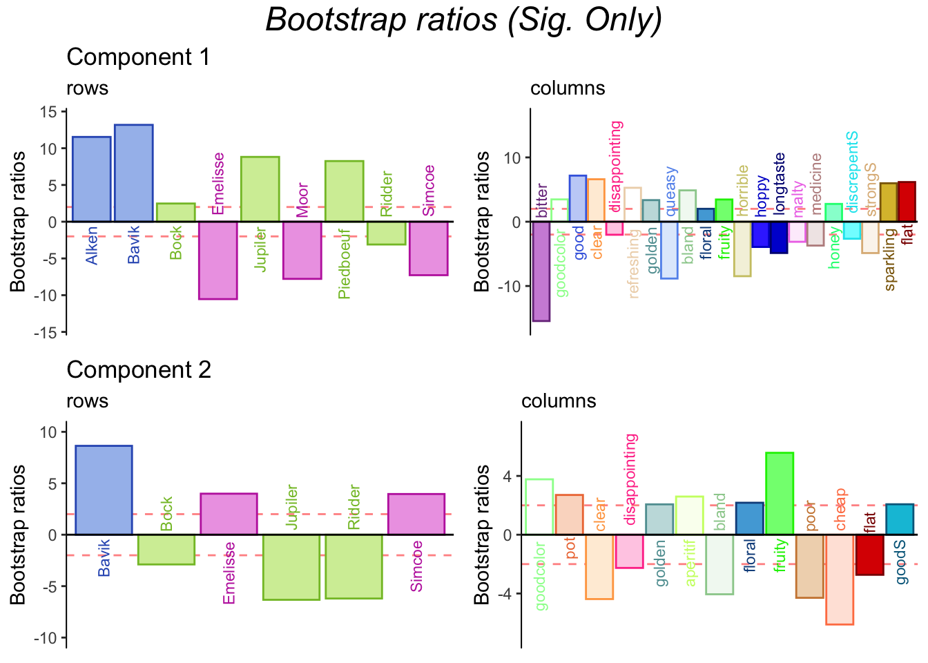
Bootstraps support contributions.

3.4 Summary

When we interpret the factor scores and loadings together, the CA revealed:

Do you prefer symmetric or asymmetric plot for your data? Symmetric, due to small effect size via eigenvalue per dimension.

Component 1

Rows: Hoppy vs Sweet

Cols: Bad taste to Good taste

Interpret: Hoppy beers have a bad taste and sweet beers have a good taste

Component 2

Rows: Sweet vs Bland

Cols: Physical characteristics

Interpret: Sweeter beers have stronger physical characteristics as opposed to bland beers