Chapter 4 Multiple Correspondence Analysis
PCA for several qualitative variables that have been disjunctively coded into 0’s and 1’s. The data set consists of observations in the rows and variables in the columns. Unlike CA, MCA only uses the symmetric map. Therefore, levels of variables close to each other on the loadings plot are chosen together.
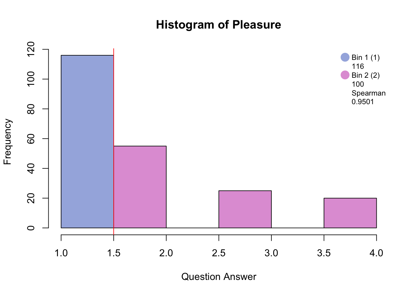
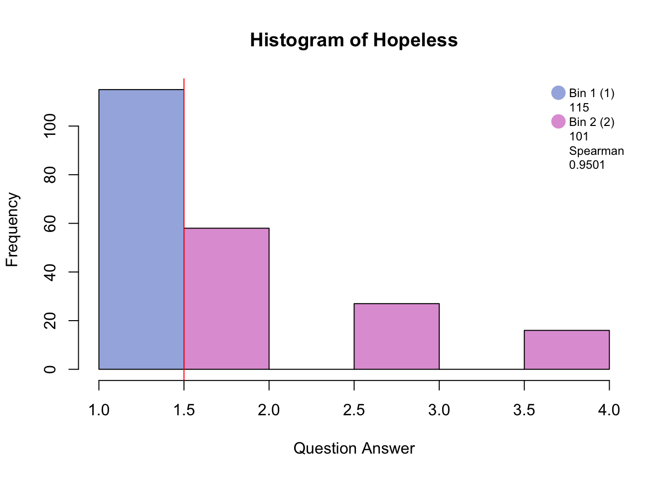
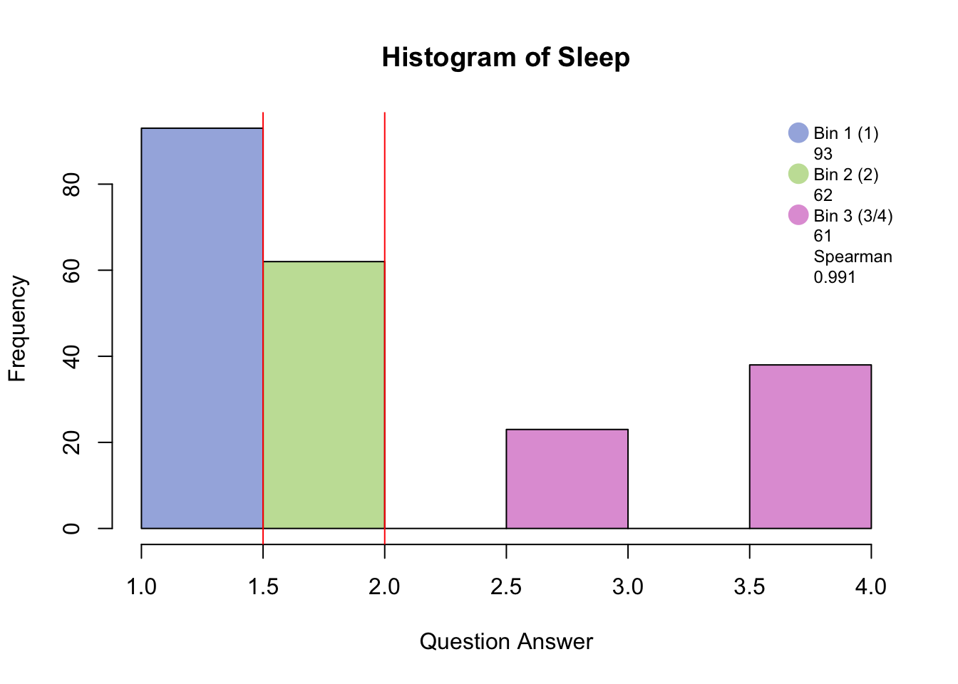
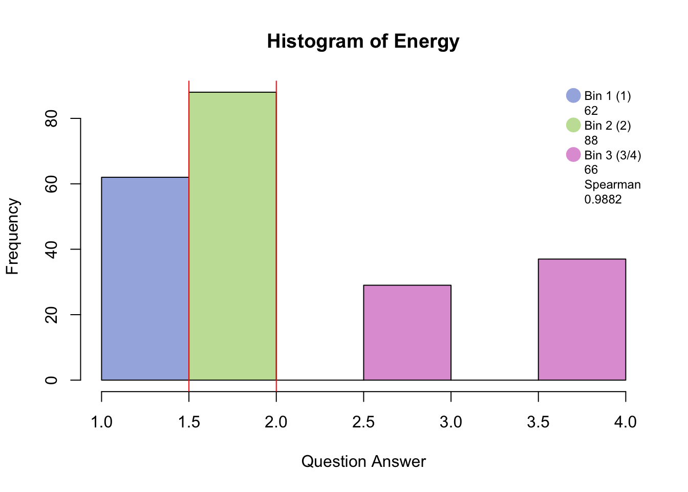
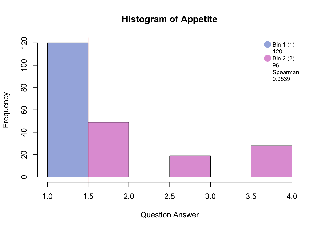
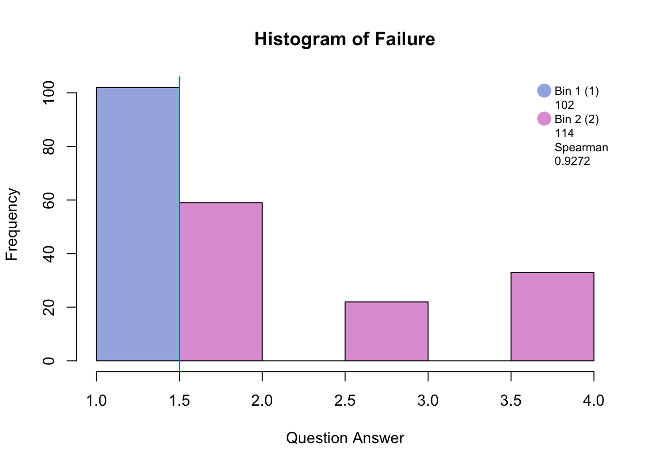
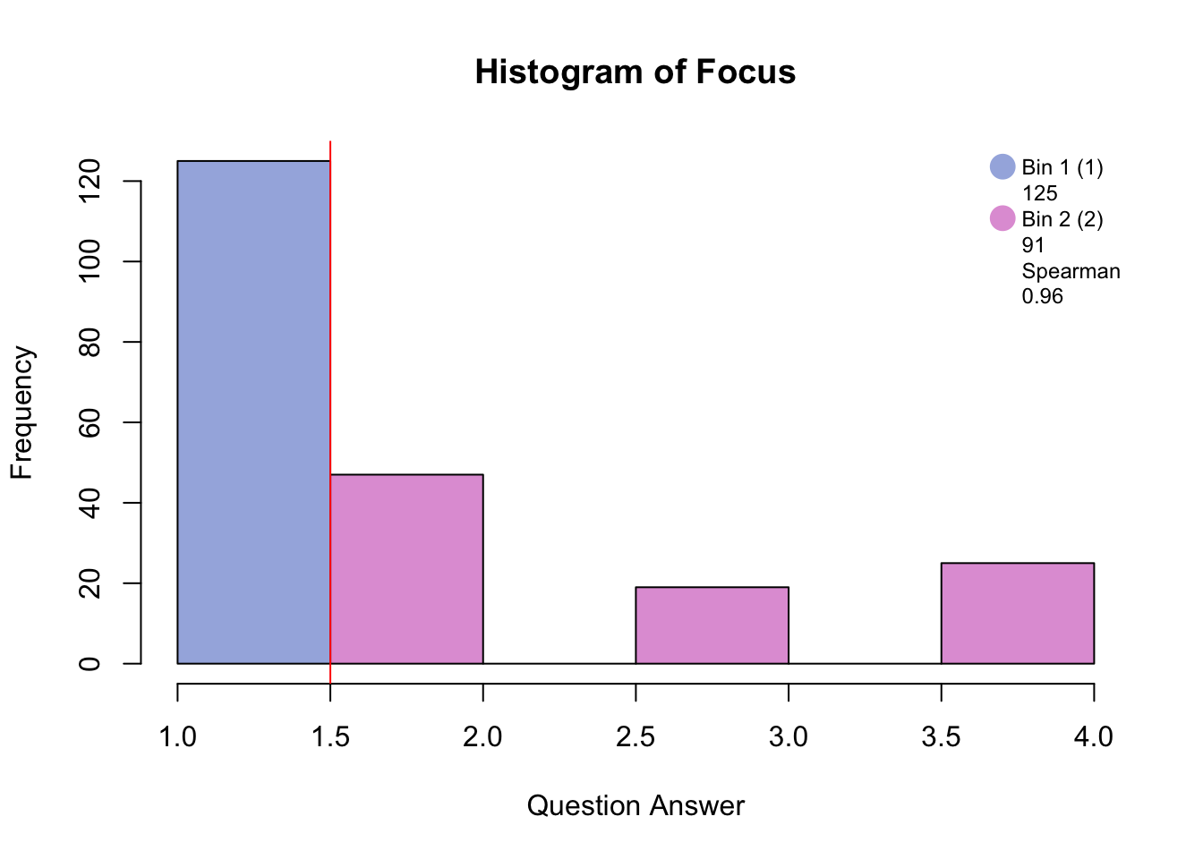
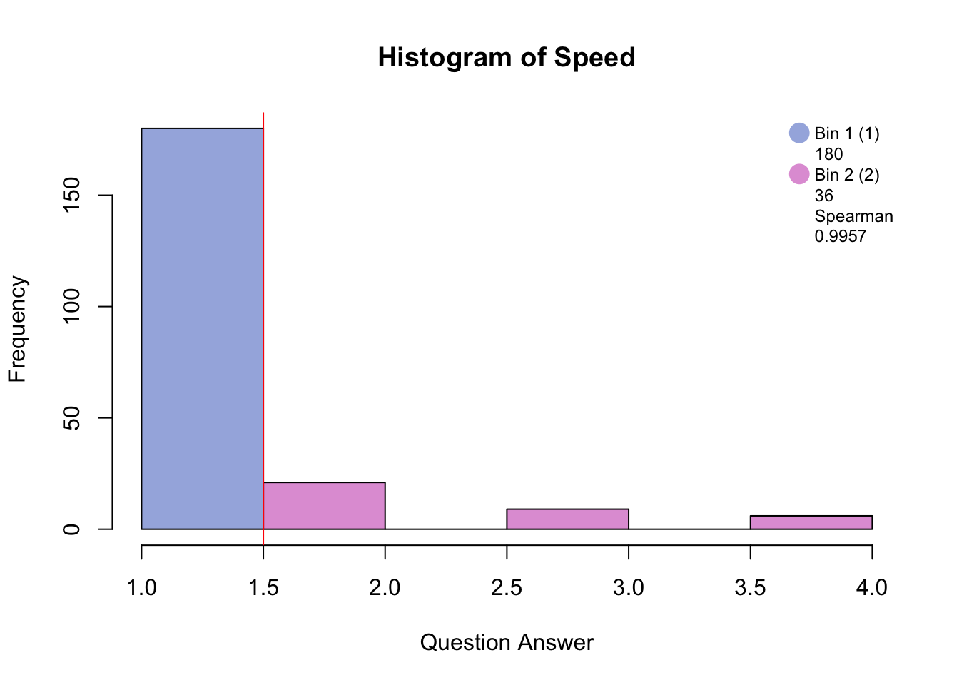
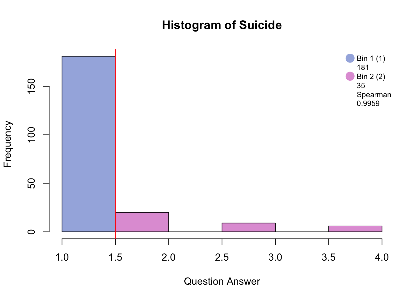
Before disjunctively coding, the data has to be either binned into quartiles/quantiles if normally distributed, or binned by eye in order to make a balanced design i.e. similar number of participants in each bin. The similarity between the raw distribution and the binned distrubtion is determined by the Spearman correlation.
MCA has the ability to separate non-linear relationships creating individual clusters from, for example, a horse shoe shaped cluster.
4.1 Binning
# Have a look and create empty SamplesMatrix and MCAdata
Question <- colnames(PHQ)[1:9]
BinMatrix <- matrix(, nrow = 9, ncol = 4)
row.names(BinMatrix) <- Question
colnames(BinMatrix) <- c("Bin 1 (1)", "Bin 2 (2)", "Bin 3 (3/4)", "Spearman")
MCAdata <- matrix(, nrow = 216, ncol = 9)
colnames(MCAdata) <- Question
row.names(MCAdata) <- c(1:216)

##Create BinMatrix and MCAdata
for (i in 1:9) {
  if (i >= 3 & i <=4){
    recode <- cut(PHQ[,i],breaks = c(min(PHQ[,1]),1.5,2,max(PHQ[,i])+1),include.lowest = T)

    #Fills MCAdata
    MCAdata[,i] <- recode

    #Fills BinMatrix (binned according to PHQ tool)
    populate <- data.frame(table(recode))
    populate <- t(populate$Freq)
    BinMatrix[i,1:3] <- populate
    BinMatrix[i,4] <- cor(PHQ[,i],as.numeric(recode), method = "spearman")

    #Creates histograms with bin lines
    Distribution <-hist(PHQ[,i], breaks = 8, col = c(rgb(48, 90, 191, 125, maxColorValue=255), rgb(132, 191, 48, 125, maxColorValue=255), NA, rgb(191, 48, 173, 125, maxColorValue=255), NA, rgb(191, 48, 173, 125, maxColorValue=255)), main = paste("Histogram of", colnames(PHQ)[i]), xlab = "Question Answer")

Distribution <- abline(v = c(1.5,2), col = "red")

Distribution <- legend("topright", legend = c(c(colnames(BinMatrix)[1],BinMatrix[i,1]), c(colnames(BinMatrix)[2],BinMatrix[i,2]), c(colnames(BinMatrix)[3], BinMatrix[i,3]), c(colnames(BinMatrix)[4], round(BinMatrix[i,4], digits = 4))),pch = 16, pt.cex = 2, cex = .75, bty = 'n', col =c(rgb(48, 90, 191, 125, maxColorValue=255), NA, rgb(132, 191, 48, 125, maxColorValue=255), NA, rgb(191, 48, 173, 125, maxColorValue=255), NA, NA, NA))
  } else {
     recode <- cut(PHQ[,i],breaks = c(min(PHQ[,1]),1.5,max(PHQ[,i])+1),include.lowest = T)

     #Fills MCAdata
     MCAdata[,i] <- recode

     #Fills BinMatrix (Binned according to PHQ tool)
     populate <- data.frame(table(recode))
    populate <- t(populate$Freq)
    BinMatrix[i,1:2] <- populate
    BinMatrix[i,3] <- NA
    BinMatrix[i,4] <- cor(PHQ[,i],as.numeric(recode), method = "spearman")

    #Creates histogram with bin line and legend
    Distribution <-hist(PHQ[,i], breaks = 8, col = c(rgb(48, 90, 191, 125, maxColorValue=255), c(rgb(191, 48, 173, 125, maxColorValue=255), rgb(191, 48, 173, 125, maxColorValue=255), rgb(191, 48, 173, 125, maxColorValue=255))), main = paste("Histogram of", colnames(PHQ)[i]), xlab = "Question Answer")

    Distribution <- legend("topright", legend = c(c(colnames(BinMatrix)[1],BinMatrix[i,1]), c(colnames(BinMatrix)[2],BinMatrix[i,2]), c(colnames(BinMatrix)[4], round(BinMatrix[i,4], digits = 4))),pch = 16, pt.cex = 2, cex = .75, bty = 'n', col =c(rgb(48, 90, 191, 125, maxColorValue=255), NA, rgb(191, 48, 173, 125, maxColorValue=255), NA, NA, NA))

    Distribution <- abline(v = 1.5, col = "red")
  }
}
##What it would have looked like without loop
#BinMatrix
## Look at the variables ----
#hist.Pleasure <- hist(PHQ[,1], breaks = 20,  main = paste("Histogram of", colnames(PHQ)[1]))
#Pleasure_recode <- cut(PHQ[,1],breaks = c(min(PHQ[,1]),1.5,2,max(PHQ[,1])+1),include.lowest = T)
#Pleasure <- data.frame(table(Pleasure_recode))
#Pleasure <- t(Pleasure$Freq)
# check the spearman's rank correlation
#PleasureCor <- cor(PHQ[,1],as.numeric(Pleasure_recode), method = "spearman")

#hist.Hopeless <- hist(PHQ[,2], breaks = 20,  main = paste("Histogram of", colnames(PHQ)[2]))
#Hopeless_recode <- cut(PHQ[,2],breaks = c(min(PHQ[,2]),1.5,2,max(PHQ[,2])+1),include.lowest = T)
#table(Hopeless_recode)
# check the spearman's rank correlation
#cor(PHQ[,2],as.numeric(Hopeless_recode), method = "spearman")

#hist.Sleep <- hist(PHQ[,3], breaks = 20,  main = paste("Histogram of", colnames(PHQ)[3]))
#Sleep_recode <- cut(PHQ[,1],breaks = c(min(PHQ[,1]),1.5,2,max(PHQ[,1])+1),include.lowest = T)
#table(Pleasure_recode)
# check the spearman's rank correlation
#cor(PHQ[,1],as.numeric(Pleasure_recode), method = "spearman")

#hist.Energy <- hist(PHQ[,4], breaks = 20,  main = paste("Histogram of", colnames(PHQ)[4]))
#hist.Appetite <- hist(PHQ[,5], breaks = 20,  main = paste("Histogram of", colnames(PHQ)[5]))
#hist.Failure <- hist(PHQ[,6], breaks = 20,  main = paste("Histogram of", colnames(PHQ)[6]))
#hist.Focus <- hist(PHQ[,7], breaks = 20, main = paste("Histogram of", colnames(PHQ)[7]))
#hist.Speed <- hist(PHQ[,8], breaks = 20, main = paste("Histogram of", colnames(PHQ)[8]))

#hist.Suicide <- hist(PHQ[,9], breaks = 20, main = paste("Histogram of", colnames(PHQ)[9]))
#Suicide_recode <- cut(PHQ[,9],breaks = c(min(PHQ[,9]),1.5,max(PHQ[,9])+1),include.lowest = T)
#Suicide <- data.frame(table(Suicide_recode))
#Suicide <- t(Suicide$Freq)
# check the spearman's rank correlation
#SuicideCor <- cor(PHQ[,9],as.numeric(Suicide_recode), method = "spearman")
#hist.Pleasure
#hist.Hopeless
#hist.Sleep
#hist.Energy
#hist.Appetite
#hist.Failure
#hist.Focus
#hist.Speed
#hist.Suicide
Binning with blue and pink has created groups of “no days” and “several days and higher.”
Binning with blue, green, and pink has created groups of “no days”, “several days”, and “more than half days/nearly every day.”
4.2 Heatmap of Loadings
#MCA heat map
corrMatBurt.list <- phi2Mat4BurtTable(MCAdata)
cor.plot.numPhi22 <- corrplot(as.matrix(corrMatBurt.list$phi2.mat), method = "number", type = "upper", tl.pos = "lt", tl.cex = .7, tl.srt = 45, addCoefasPercent = TRUE, number.cex = .7)
cor.plot.fullPhi22 <- corrplot(as.matrix(corrMatBurt.list$phi2.mat), method = "ellipse", type = "lower", add = TRUE,
                          diag = FALSE, tl.pos = "n", cl.pos = "n")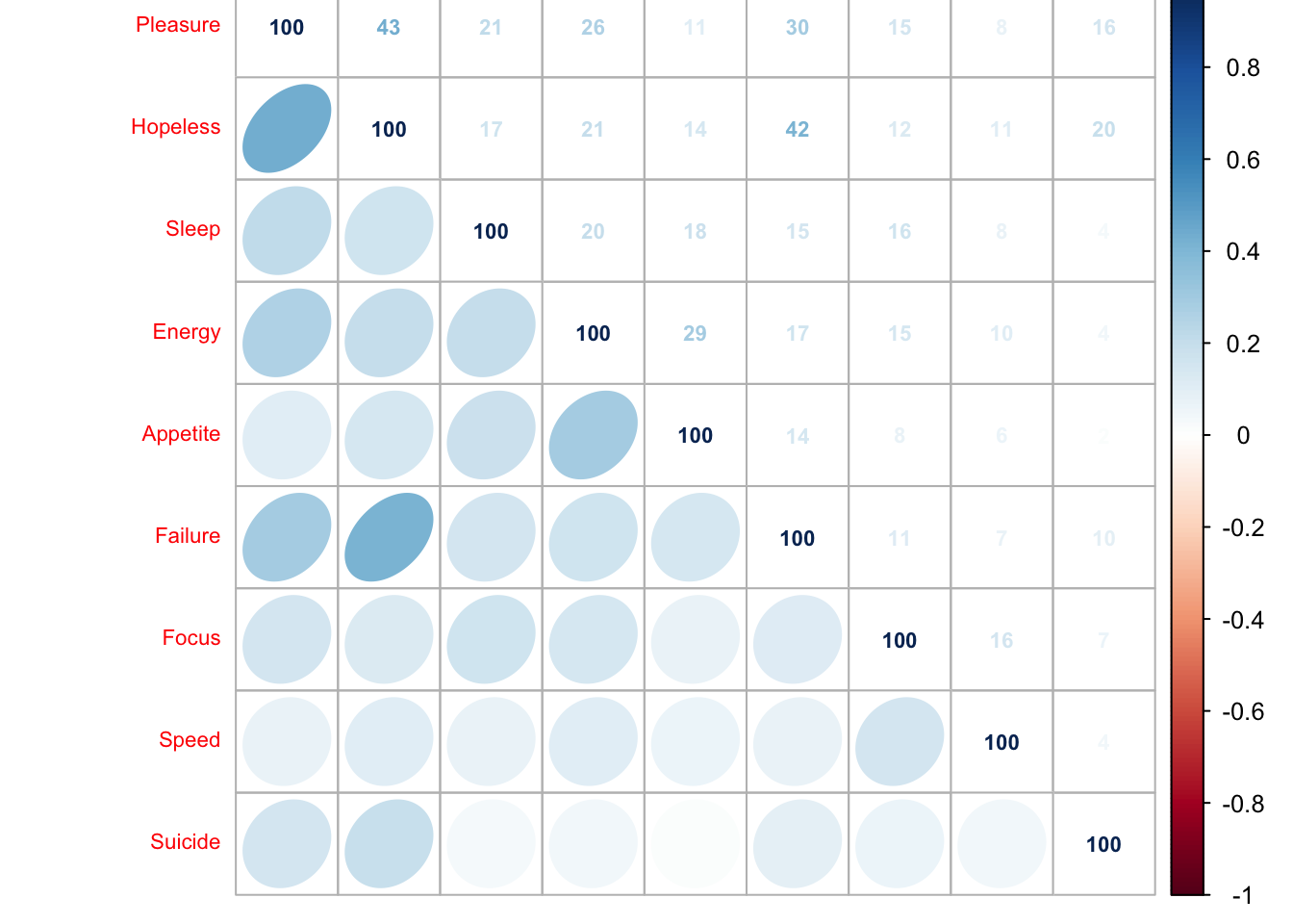
#a0001a.corMat.phi2 <- recordPlot()

# We need correlation to compare with PCA
corrMatBurt.list <- phi2Mat4BurtTable(MCAdata)
cor.plot.numPhi2 <- corrplot(as.matrix(sqrt(corrMatBurt.list$phi2.mat)), method = "number", type = "upper", tl.pos = "lt", tl.cex = .7, tl.srt = 45, addCoefasPercent = TRUE, number.cex = .7)
cor.plot.fullPhi2 <- corrplot(as.matrix(sqrt(corrMatBurt.list$phi2.mat)), method = "ellipse", type = "lower", add = TRUE,
                          diag = FALSE, tl.pos = "n", cl.pos = "n")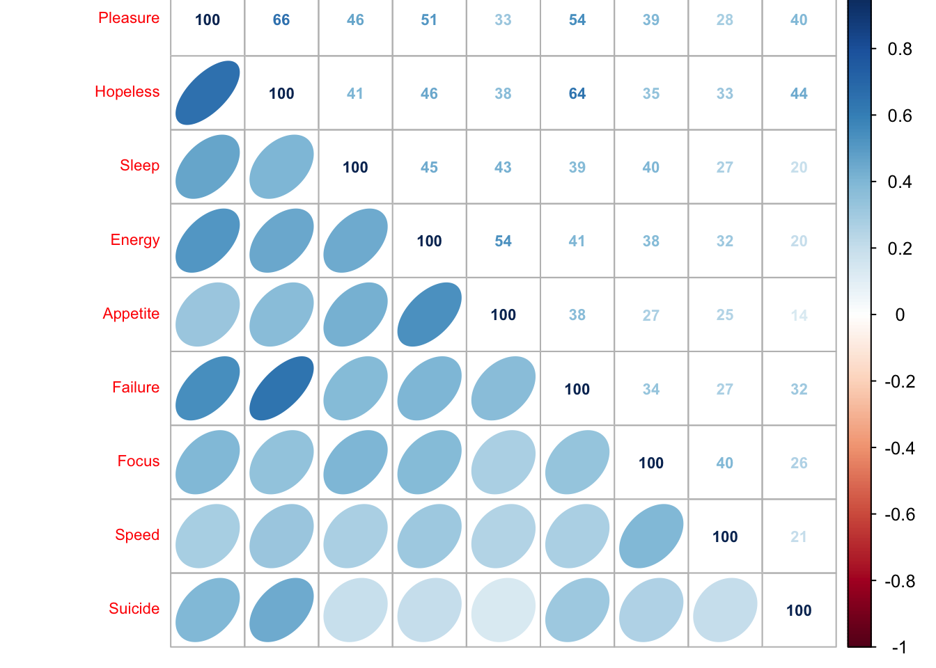
This heat map shows that the disjunctively coded data is positively correlated i.e. when one variable increases the other is likely to also increase and visa versa.
4.3 Analysis
#ONLY RUN THIS ONCE!!!!

MCAdata <- makeNominalData(MCAdata)
resMCA <- epMCA(MCAdata,
                make_data_nominal = FALSE,
                DESIGN = GroupingVaribles$memoryGroups,
                graphs = FALSE)
4.3.1 The Data Pattern
4.3.2 Inference
resMCA.inf <- InPosition::epMCA.inference.battery(MCAdata,
                                make_data_nominal = FALSE,
                                DESIGN = GroupingVaribles$memoryGroups,
                                graphs =  FALSE) # TRUE first pass only
## [1] "It is estimated that your iterations will take 0.02 minutes."
## [1] "R is not in interactive() mode. Resample-based tests will be conducted. Please take note of the progress bar."
## ===========================================================================4.3.3 Scree Plot
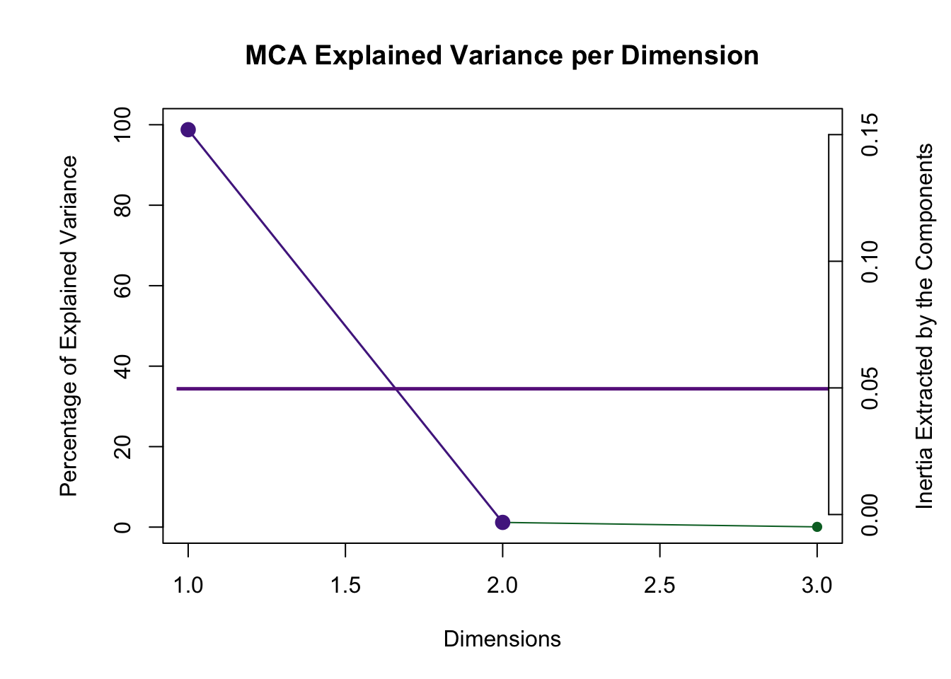
Dimension 1 is reliable and aboe the Kaiser line.
4.3.4 Row Factor Scores
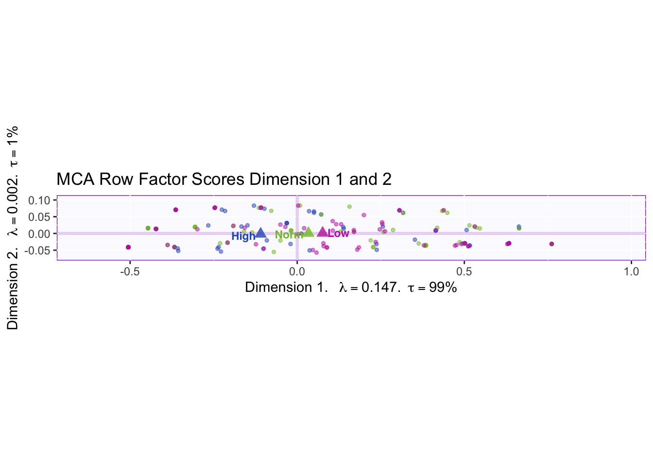
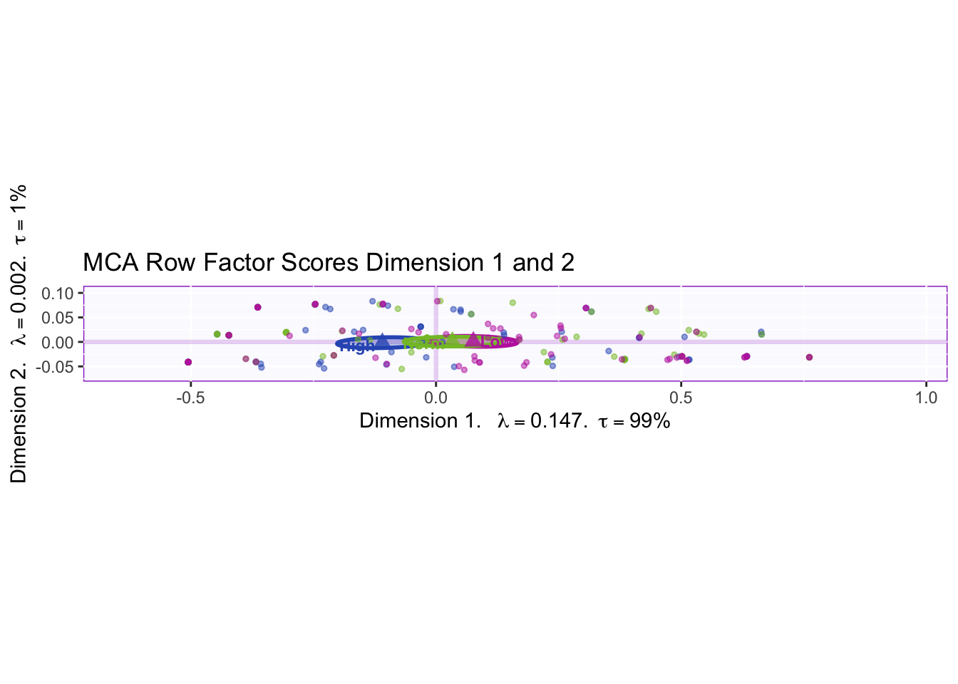
There is a null effect between the three memory groups.
4.3.5 Column Loadings
#Colors for Variables (Grouped)
#ColorTheme <- prettyGraphsColorSelection(n.colors = 9)
t <- 1
for (k in 1:3) {
  if ( k <= 2){
  p <- (2*k)
  resMCA.inf$Fixed.Data$Plotting.Data$fj.col[t:p,] <- ColorTheme[k]
  t <- (t + 2)
  }
  if (k == 3){
    p <- (1 + (2*k))
    resMCA.inf$Fixed.Data$Plotting.Data$fj.col[t:p,] <- ColorTheme[k]
    t <- (t +3)
  }
}

for (k in 4:9) {
  if (k == 4){
    p <- (2 + (2*k))
    resMCA.inf$Fixed.Data$Plotting.Data$fj.col[t:p,] <- ColorTheme[k]
    t <- (t +3)
  }
   if ( k >=5){
  p <- (2+(2*k))
  resMCA.inf$Fixed.Data$Plotting.Data$fj.col[t:p,] <- ColorTheme[k]
  t <- (t + 2)
  }
}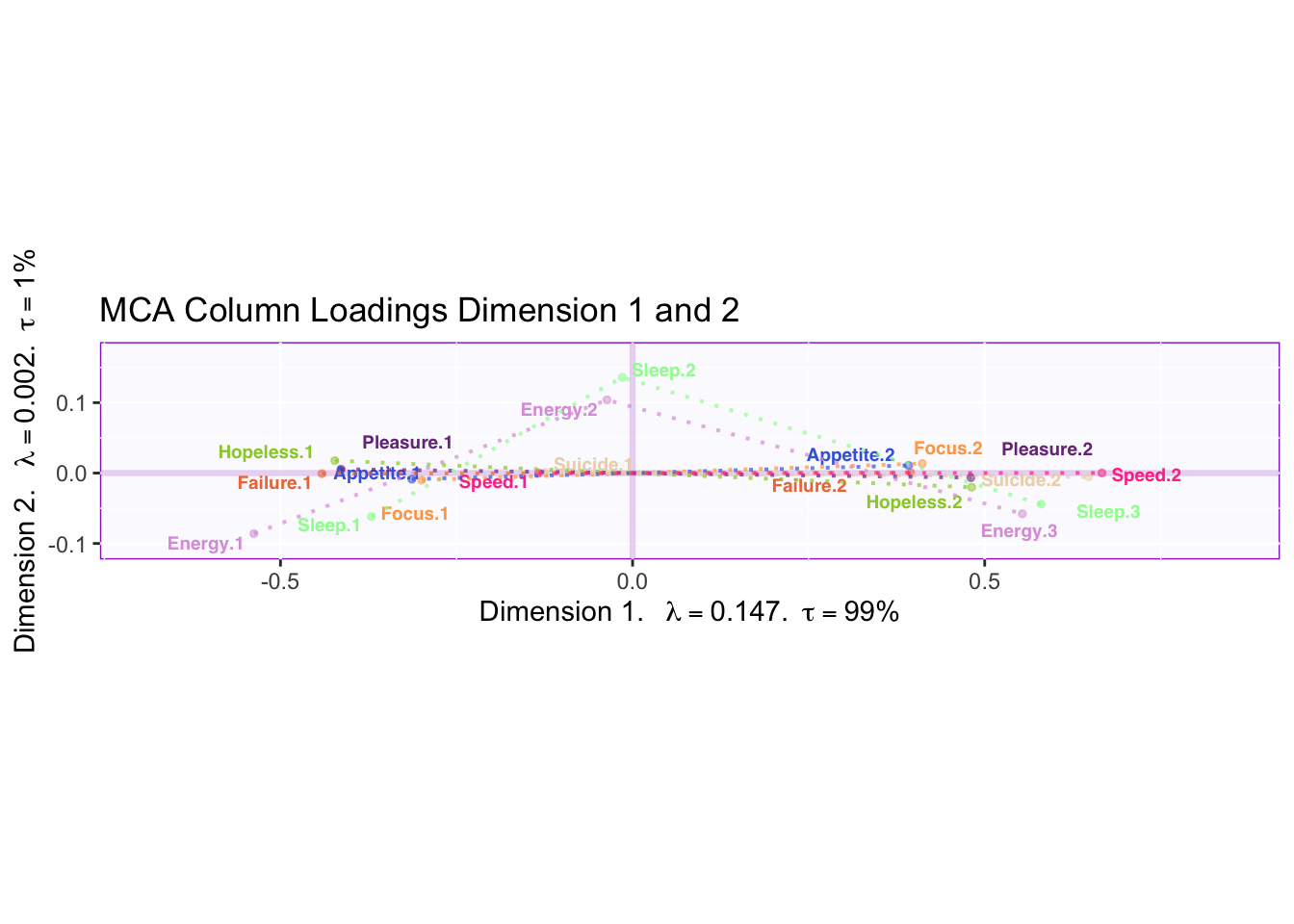
Dimension 1 is capturing the extreme differences while Dimension 2 is capturing the moderate answer of “several days.” However, “several days” is more similar to “no days” than “more than half the days.”
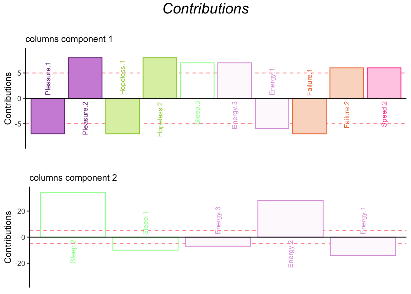
4.3.6 Contributions
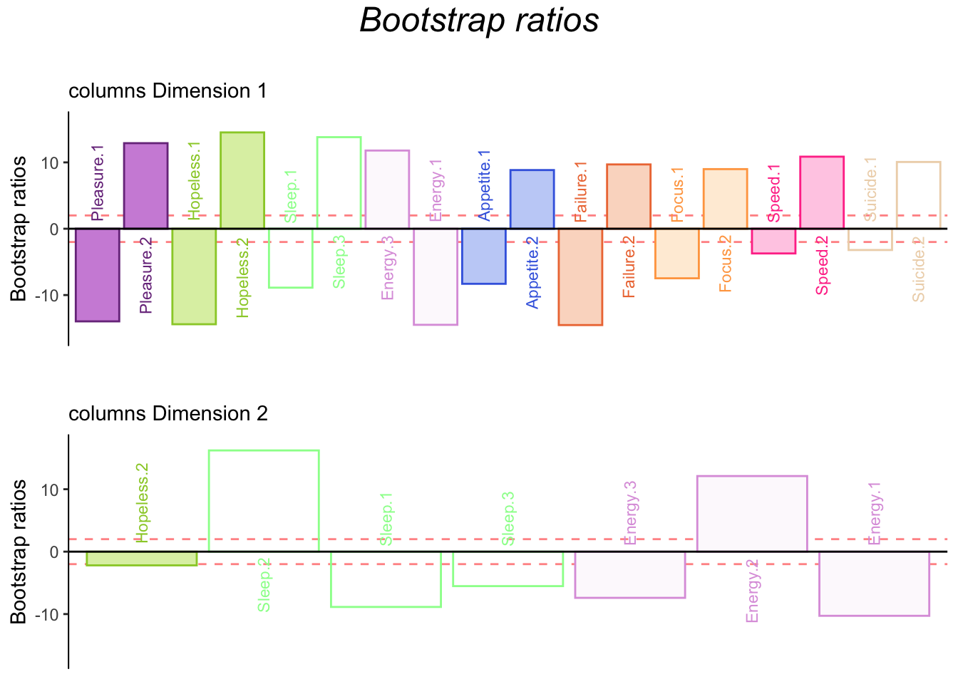
4.3.7 Bootstrap Ratios
4.4 Summary
When we interpret the factor scores and loadings together, the MCA revealed:
Dimension 1:
Rows: No difference
Columns: Some participants score “no days” on pleasure, hopeless, energy, and failure while some participants score “several days or higher” on pleasure, hopeless, sleep, energy, failure, and speed.
Dimension 2:
Rows: No difference.
Columns: Some pariticpants score “no days” on sleep.