Chapter 7 Multiple Factor Analysis
MFA is used on three or more data tables of the same observations (participants).
First a PCA without scaling is performed on the individual tables of the same observations, then divide all tables by their respective 1st singular value from the diagonal matrix from PCA (this is the weighting step/normalization), then concatenate all weighted tables (compromise), and finally do a GPCA on the compromise.
GPCA uses GSVD which uses different constraints than normal SVD. GSVD takes into consideration the masses for the observations and the squared weights for the different tables i.e. squared 1st singular value of each PCA for the respective talbe. As noted by Dr. Abdi equal masses are often assigned to each observation i.e. 1 divided the number of observations. Even with these new constraints they must equal the identity matrix. If the masses and weights are equivalent then GSVD reduces to the normal SVD.
7.1 Data sets: PHQ, OSIQ, and BFI
The Big Five Inventory measures different personality traits on a scale from 1 i.e. “completely disagree” to 5 i.e “completely agree”. The neutral option is located at 3.
The rows are the 216 participants (same number as PHQ and OSIQ) and 44 quantitative measures (8 Extraversion, 9 Agreeableness, 9 Conscientiousness, 8 Neuroticism, 10 Openness).
| Ex1 | Ex2 | Ex3 | Ex4 | Ex5 | Ex6 | Ex7 | Ex8 | Ag1 | Ag2 | Ag3 | Ag4 | Ag5 | Ag6 | Ag7 | Ag8 | Ag9 | Co1 | Co2 | Co3 | Co4 | Co5 | Co6 | Co7 | Co8 | Co9 | Ne1 | Ne2 | Ne3 | Ne4 | Ne5 | Ne6 | Ne7 | Ne8 | Op1 | Op2 | Op3 | Op4 | Op5 | Op6 | Op7 | Op8 | Op9 | Op10 |
|---|---|---|---|---|---|---|---|---|---|---|---|---|---|---|---|---|---|---|---|---|---|---|---|---|---|---|---|---|---|---|---|---|---|---|---|---|---|---|---|---|---|---|---|
| 5 | 2 | 4 | 4 | 4 | 3 | 3 | 3 | 2 | 4 | 5 | 3 | 3 | 3 | 3 | 4 | 4 | 5 | 4 | 5 | 2 | 3 | 4 | 4 | 4 | 3 | 3 | 4 | 5 | 5 | 2 | 1 | 3 | 4 | 2 | 5 | 3 | 4 | 2 | 3 | 5 | 5 | 3 | 4 |
| 2 | 2 | 4 | 4 | 4 | 3 | 2 | 2 | 3 | 4 | 4 | 4 | 4 | 4 | 4 | 4 | 5 | 3 | 2 | 4 | 3 | 4 | 4 | 4 | 4 | 4 | 2 | 2 | 4 | 3 | 2 | 2 | 2 | 2 | 5 | 5 | 5 | 5 | 4 | 4 | 4 | 5 | 4 | 4 |
| 3 | 2 | 4 | 3 | 2 | 2 | 2 | 5 | 1 | 1 | 1 | 5 | 1 | 1 | 1 | 1 | 4 | 1 | 1 | 2 | 4 | 1 | 5 | 4 | 1 | 5 | 5 | 5 | 1 | 5 | 5 | 5 | 5 | 2 | 5 | 4 | 1 | 3 | 4 | 1 | 1 | 5 | 5 | 2 |
| 2 | 2 | 2 | 2 | 2 | 3 | 2 | 4 | 2 | 5 | 5 | 3 | 3 | 3 | 4 | 4 | 4 | 3 | 4 | 5 | 2 | 2 | 4 | 4 | 4 | 5 | 5 | 3 | 2 | 4 | 3 | 2 | 2 | 3 | 4 | 5 | 5 | 5 | 3 | 4 | 2 | 5 | 4 | 5 |
| 4 | 3 | 2 | 3 | 3 | 3 | 4 | 4 | 2 | 4 | 5 | 2 | 2 | 3 | 4 | 4 | 5 | 5 | 1 | 5 | 1 | 2 | 5 | 4 | 5 | 2 | 2 | 3 | 4 | 3 | 4 | 3 | 4 | 3 | 3 | 4 | 4 | 4 | 4 | 5 | 4 | 4 | 5 | 2 |
| 5 | 4 | 2 | 4 | 4 | 4 | 4 | 5 | 2 | 4 | 5 | 4 | 4 | 4 | 2 | 2 | 4 | 4 | 4 | 5 | 5 | 2 | 4 | 4 | 5 | 2 | 4 | 4 | 4 | 5 | 2 | 4 | 1 | 2 | 4 | 4 | 4 | 2 | 2 | 5 | 4 | 2 | 5 | 4 |
7.2 Analysis
## [1] "Preprocessed the Rows of the data matrix using:  None"
## [1] "Preprocessed the Columns of the data matrix using:  Center_1Norm"
## [1] "Preprocessed the Tables of the data matrix using:  MFA_Normalization"
## [1] "Preprocessing Completed"
## [1] "Optimizing using:  None"
## [1] "Processing Complete"
7.2.1 Correlation Plot
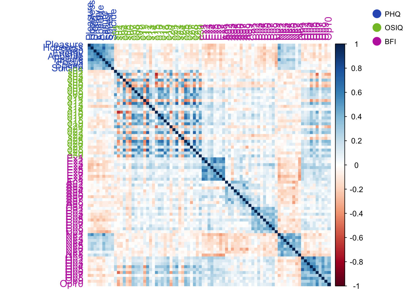
The correlation plot shows that neurtoicism is positively correlated with the PHQ and the PHQ is negatively correlated with almost everything else.
The BFI is positvely correlated with itself, except for neuroticism.
7.2.2 RV Matrix Correlation and Weights for Each Table
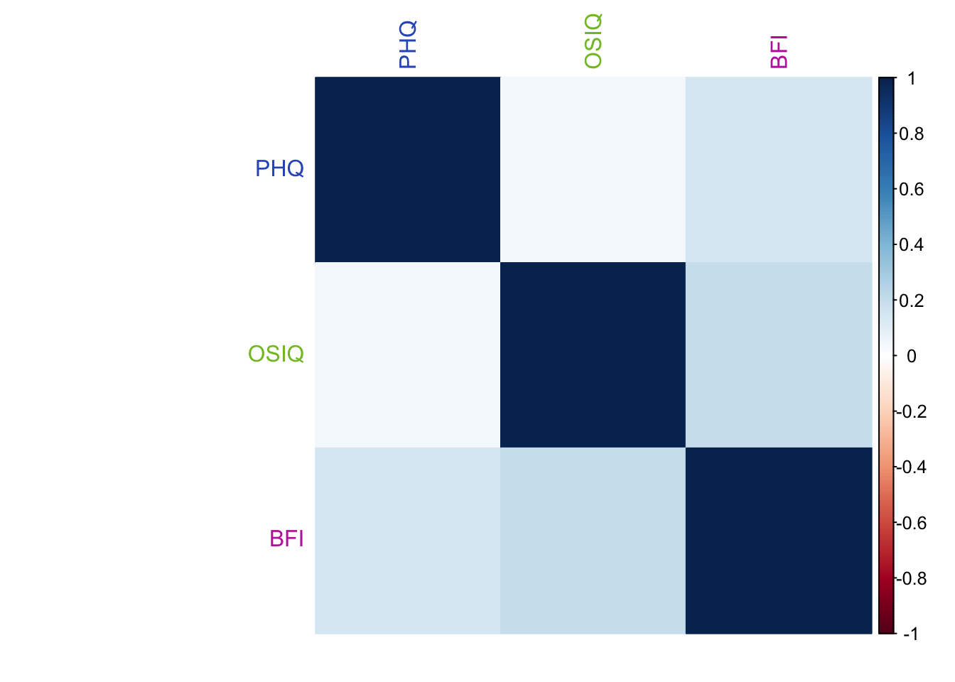
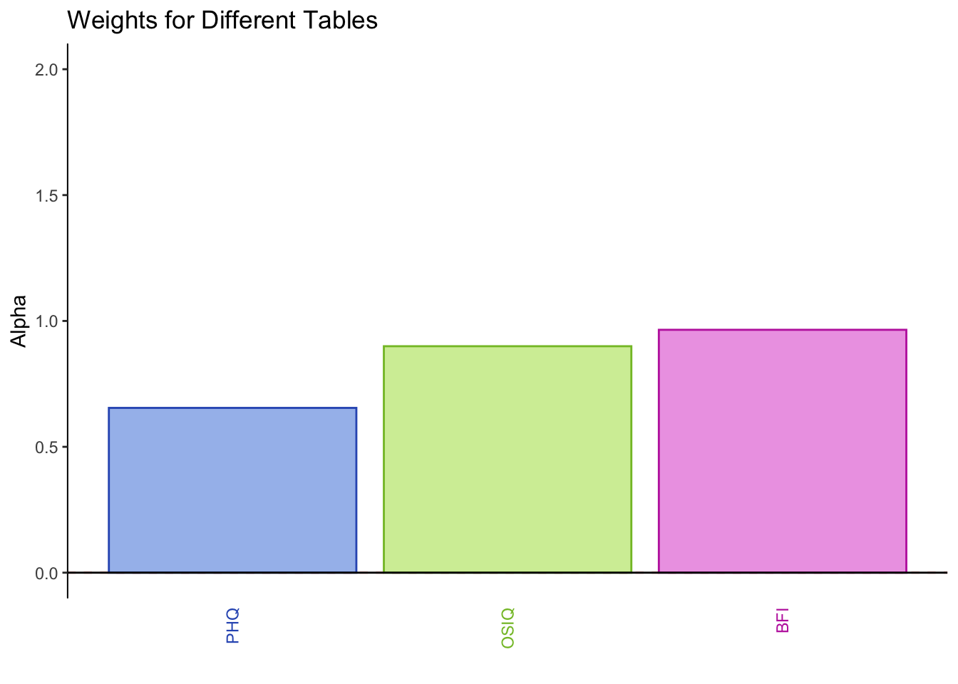
PHQ and OSIQ are overall positively correlated, but not as much as PHQ and the BFI (neuroticism). The BFI and OSIQ are positively correlated higher than PHQ and BFI.
The weights for each table are obtained from the 1st singular value (stored in the diagonal matrix derived from SVD) of its PCA. In this instance, PHQ has the smallest singular value, OSIQ has the 2nd smallest, and BFI has the largest.
7.2.3 Scree Plot
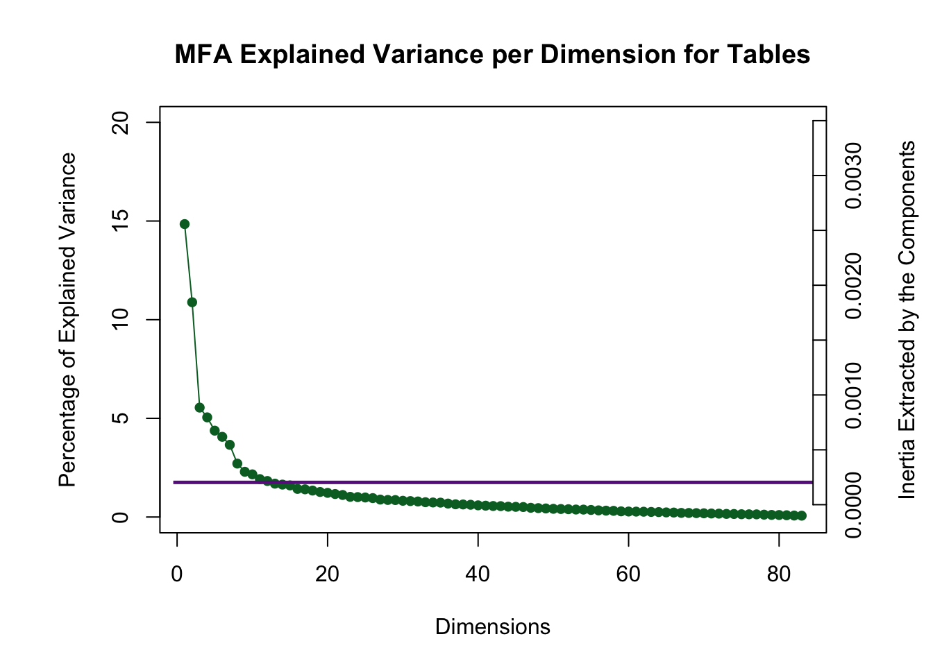
There are many dimensions above the Kaiser line, but in this instance only the first three analyzed due to the 3rd and 4th creating an eigen-plane (they would need to be interpreted together) and the 5th, 6th, and 7th creating an eigen-cube.
7.2.4 Global Factor Scores of the Rows: How the rows are projected onto the space from the perspective of all tables (compromise)
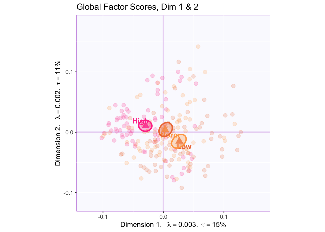
There is reliable separation between all three groups in dimension 1 ( high (-) vs. normal (origin) vs. low (+)) and dimension 2 (high (+) vs. low (-)).
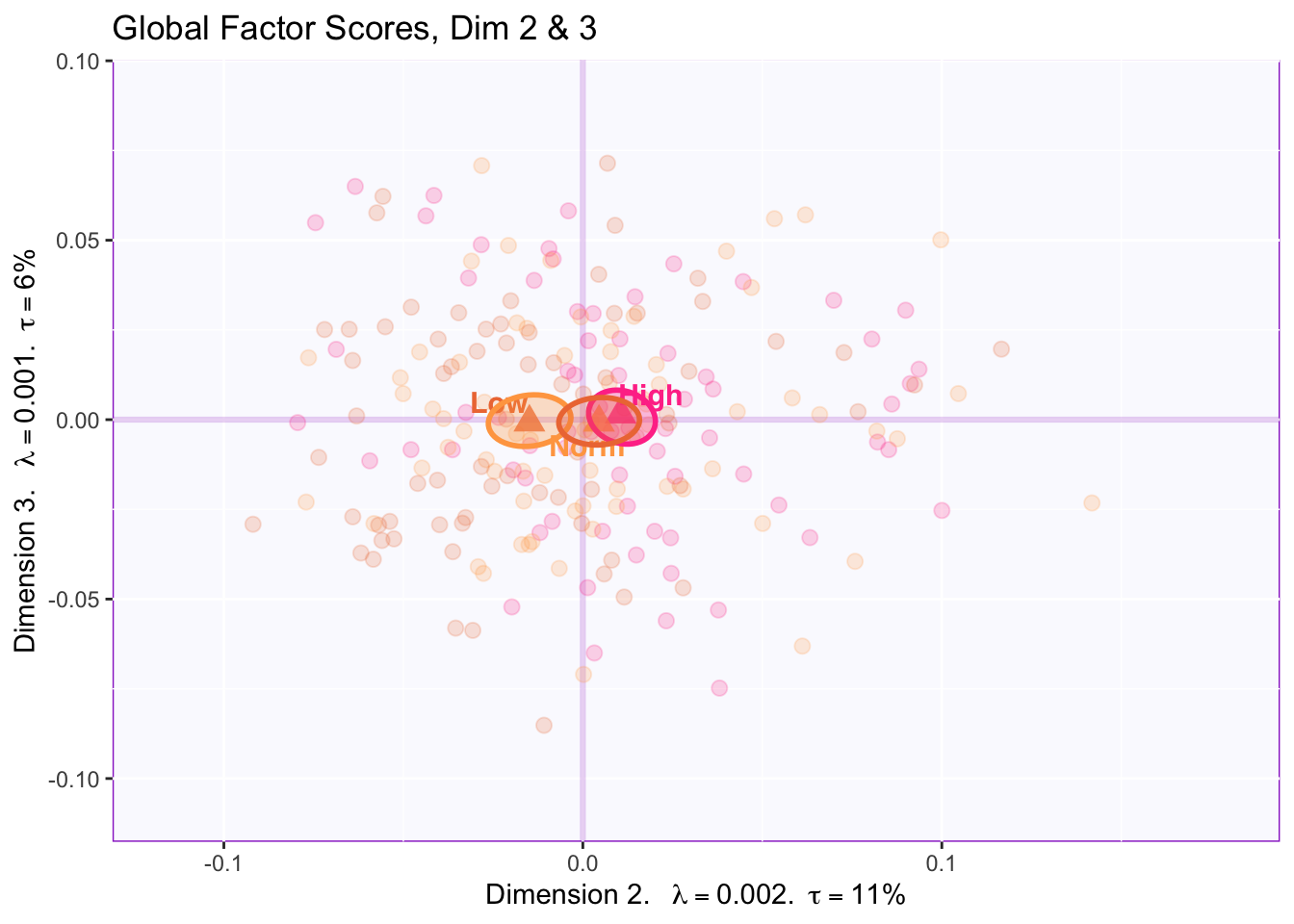
There is NOT a reliable difference between groups in dimension 3.
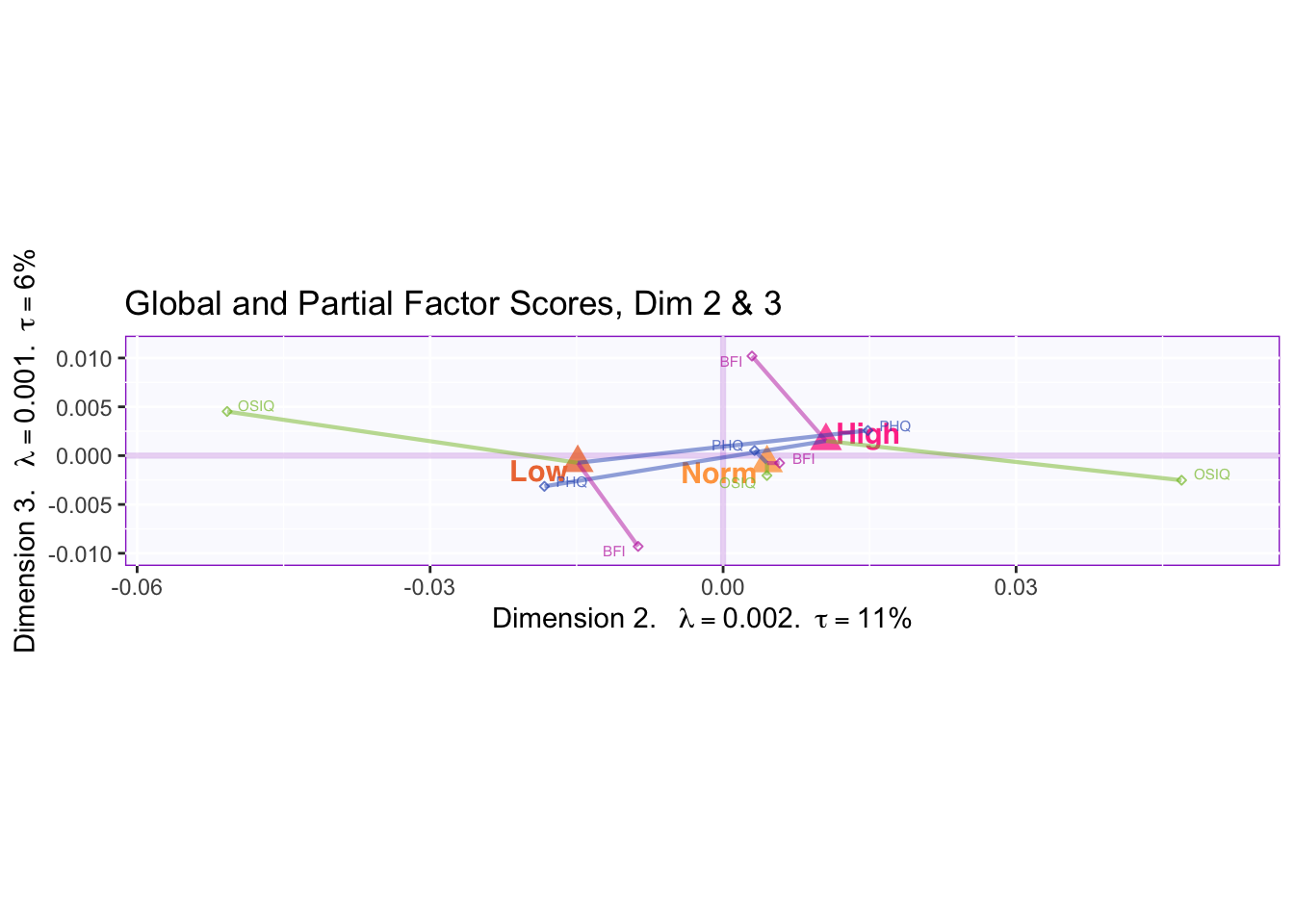
7.2.5 Mean Global Factor Scores with Partial Factor Scores
F_j <- resMFA$mexPosition.Data$Table$partial.fi.array
alpha_j <- 1/sqrt(resMFA$mexPosition.Data$Compromise$compromise.eigs)

#Finds number of tables
code4Groups <- as.numeric(unique(t(TableMembership)))
nK <- length(code4Groups)

# creates empty array for F_k
F_k <- array(0, dim = c(dim(F_j)[[1]], dim(F_j)[[2]],nK))
dimnames(F_k) <- list(dimnames(F_j)[[1]],
  dimnames(F_j)[[2]], code4Groups)
alpha_k <- rep(0, nK)
names(alpha_k) <- code4Groups
Fa_j <- F_j
# A horrible loop (Frist Normalization)
for (j in 1:dim(F_j)[[3]]){
  Fa_j[,,j] <- F_j[,,j] * alpha_j[j]
  }

# Another horrible loop (double normalization)
for (k in 1:nK){
alpha_k[k] <- sum(alpha_j[k])
F_k[,,k] <- (1/alpha_k[k])*apply(Fa_j[,,k],c(1,2),sum)
}

colnames(F_k)<-c(paste0('Dimension ',1:ncol(F_k)))

meanfk <-
  apply(F_k, c(2,3), FUN = function(x){
  aggregate(x, by = list(GroupingVaribles$memoryGroups), mean)$x
  })

for (k in 1:2) {
plot1.mean <- createFactorMap(lxy.1.means, constraints = minmaxHelper4Partial(lxy.1.means, meanfk,axis1 = k,axis2 = (k+1)),
                              axis1 = k, axis2 = k+1,
                              col.points = colorslxly[rownames(lxy.1.means),],
                              col.labels = colorslxly[rownames(lxy.1.means),],
                              title = paste("Global and Partial Factor Scores, Dim", k, "&", k+1),
                              cex = 4,
                              pch = 17,
                              alpha.points = 0.8)


map4PFS <- createPartialFactorScoresMap(factorScores = lxy.1.means,
partialFactorScores = meanfk,
axis1 = k, axis2 = k+1,
colors4Items = resMFA$Plotting.Data$fi.col, colors4Blocks = SurveyColors, names4Partial = c("PHQ", "OSIQ", "BFI")) # font.labels = 'bold')

fi.labels <- createxyLabels.gen(k,k+1,
                             lambda = resMFA$mexPosition.Data$Table$eigs,
                             tau = round(resMFA$mexPosition.Data$Compromise$compromise.t),
                             axisName = "Dimension "
                             )

d2.partialFS.map.byCategories <- plot1.mean$zeMap +
map4PFS$mapColByBlocks + fi.labels
print(d2.partialFS.map.byCategories)
#d2.partialFS.map.byCategories <- recordPlot()
}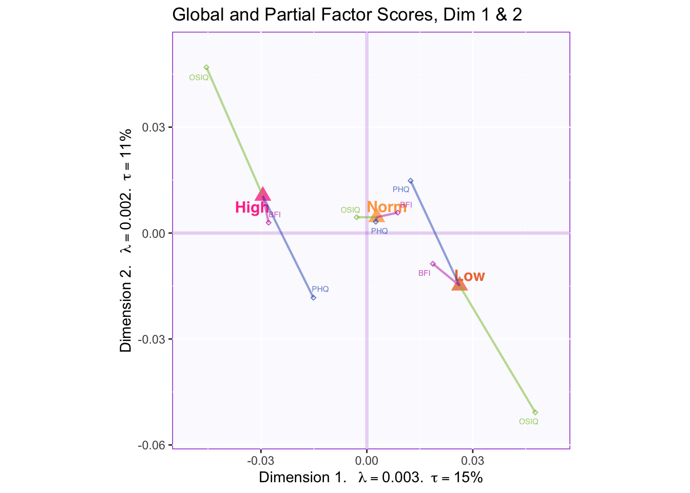
In the first two dimensions we can see that OSIQ partial factor scores are contributing the most to the difference in the mean global factor scores of the memory groups.
We can see when comparing dimensions 2 and 3 that PHQ partial factor scores are pulling the mean global factor scores together. BFI partial factor scores are found contributing to the difference between the mean global factor scores in dimension 3.
7.2.6 Significantly Contributing Loadings
Fj <- resMFA$mexPosition.Data$Table$Q
ctrj <- resMFA$mexPosition.Data$Table$cj
signed.ctrj <- ctrj * sign(Fj)

for (k in 1:2) { #(k in 1:(n-1) where "n" is the number of desired dimensions)
#Gets coordinates for contributions above threshold
CtrjAbove <- which((round(100*signed.ctrj[,k:(k+1)]) > 100/nrow(signed.ctrj)), arr.ind = TRUE)
#Gets coordinates for contributions below threshold
CtrjBelow <- which((round(100*signed.ctrj[,k:(k+1)]) < -100/nrow(signed.ctrj)), arr.ind = TRUE)
#Combines all coordinates into one vector
AllSigCtrj1 <- c(CtrjAbove, CtrjBelow)

#Remove duplicates after the first attempt----
n_occurWithDuplicates <- data.frame(table(AllSigCtrj1)) #gives a dataframe of how many times each id occured in the data
NumberOfDubplicates <- sum(n_occurWithDuplicates$Freq-1) #gives the number of duplicates, if more 0 remove # from beginning of loop
for (i in 1:NumberOfDubplicates) { #for-loop removing duplicates
y <- anyDuplicated(AllSigCtrj1)
AllSigCtrj1 <- AllSigCtrj1[-y]
   }
n_occurNoDuplicates <- data.frame(table(PHQ$row.names))  #shows there are no duplicates reamining

#Gets values for coordinates for signficant loadings in given dimensions
FSC1 <- resMFA$mexPosition.Data$Table$Q[AllSigCtrj1,k:(k+1)]
#Gets colors for signficant loadings
ColorsSigCtrj <- resMFA$Plotting.Data$fj.col[AllSigCtrj1,1]


#Plot it!
Blah<- createFactorMap(FSC1,
                      title = paste("Loadings, Dim", k, "&", k+1),
                      axis1 = 1, axis2 = 2,
                      col.points = ColorsSigCtrj,
                      col.labels = ColorsSigCtrj,
                      alpha.points = 0.5,
                      text.cex = 3,
                      )

fi.labels <- createxyLabels.gen(k,k+1,
                             lambda = resMFA$mexPosition.Data$Table$eigs,
                             tau = round(resMFA$mexPosition.Data$Compromise$compromise.t),
                             axisName = "Dimension "
                             )

PlotBlah <- Blah$zeMap_background + Blah$zeMap_dots + Blah$zeMap_text + fi.labels
print(PlotBlah)
#PlotBlah <- recordPlot()
}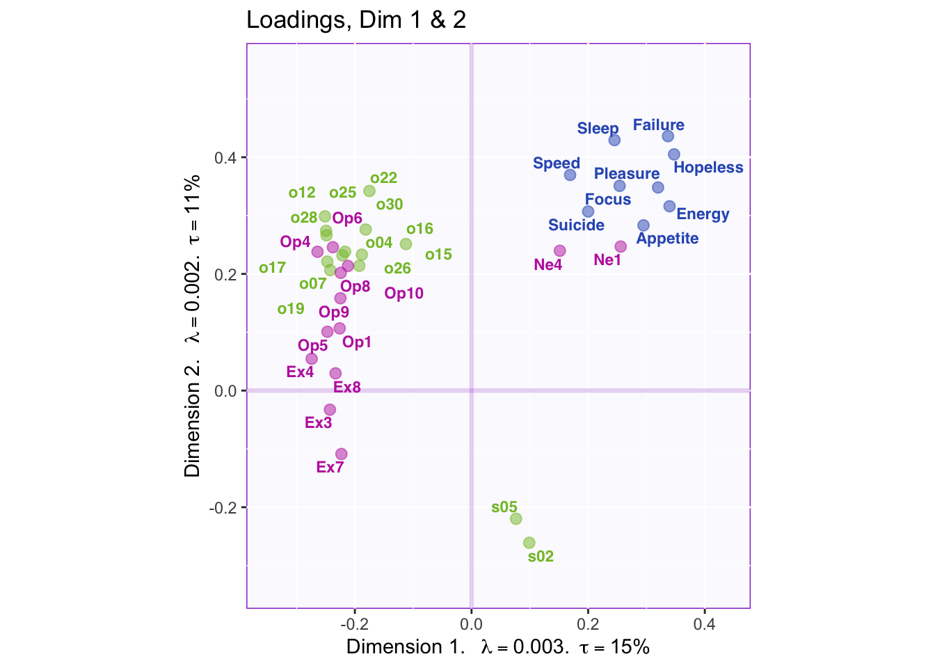
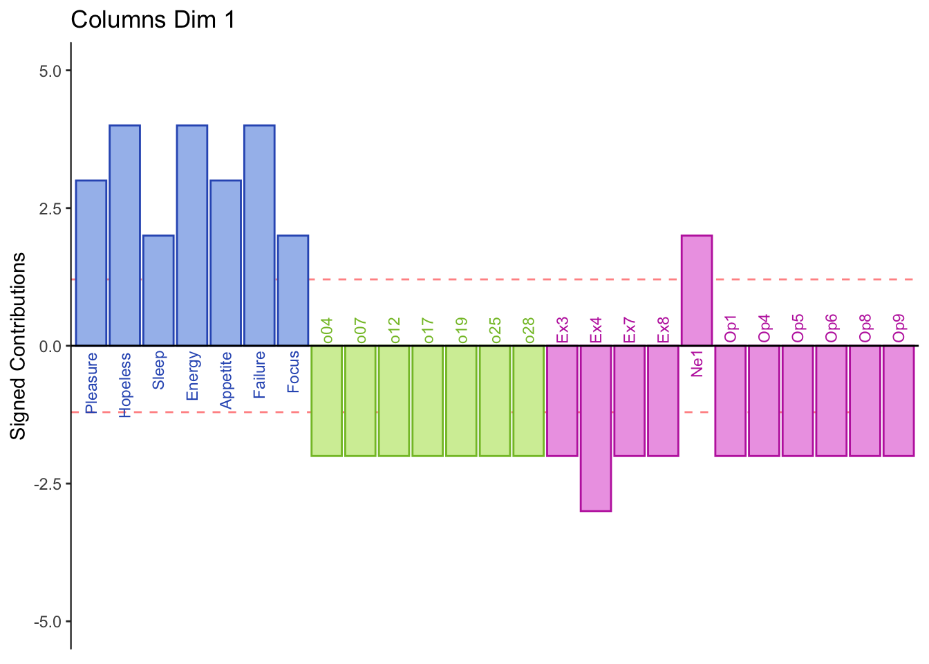
Dimension 1: PHQ, Neuroticism, and spatial 5 and 2 (+) vs. object, openness, and extroversion
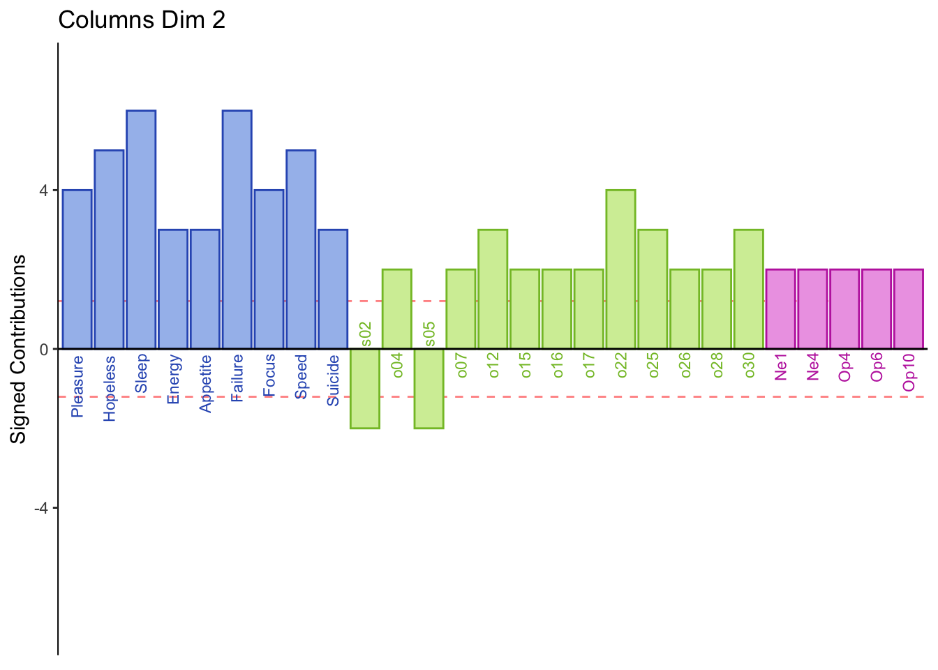
Dimension 2: Extroversion and sptial (-) vs openness, object, PHQ, and neuroticism (+)
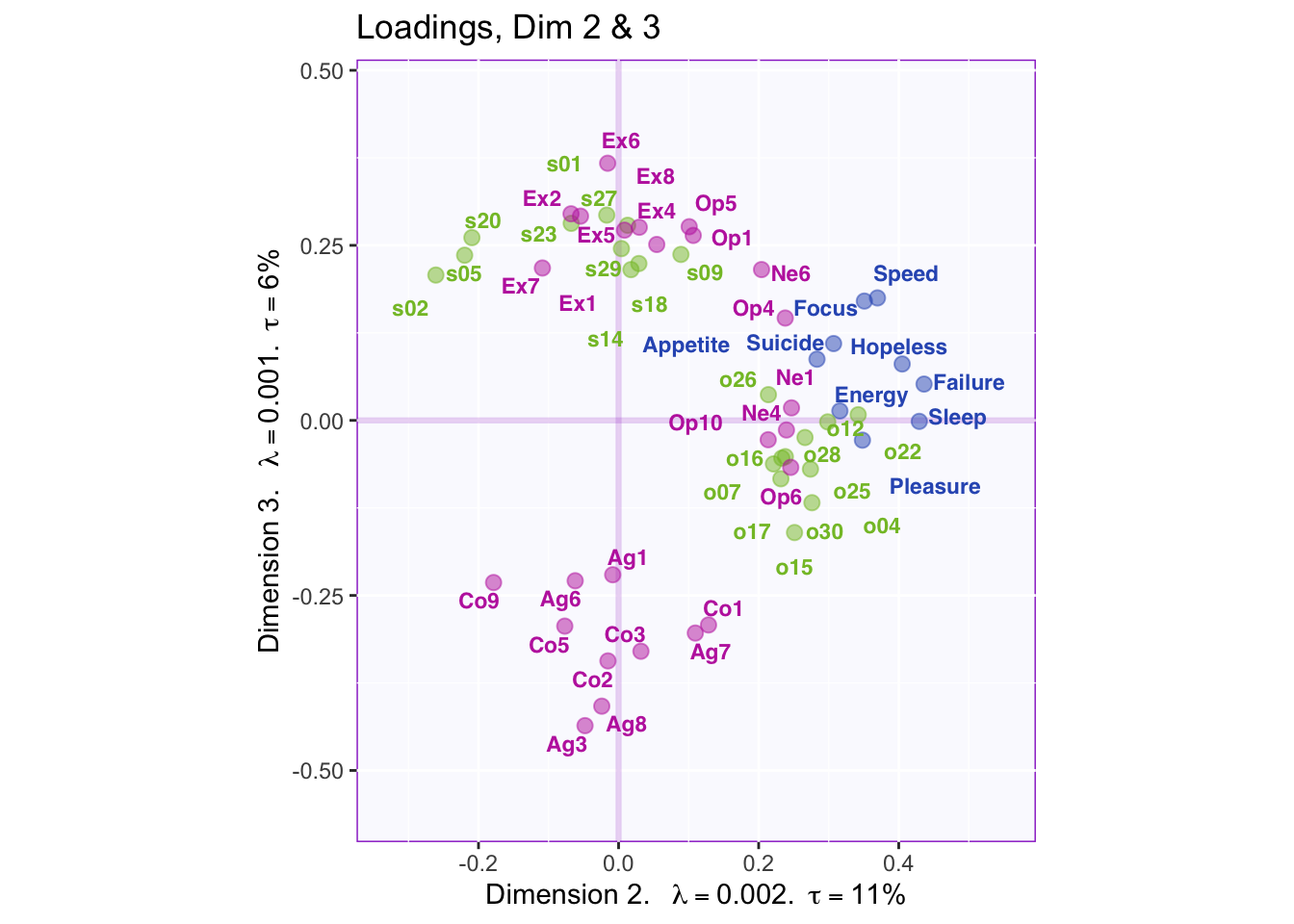
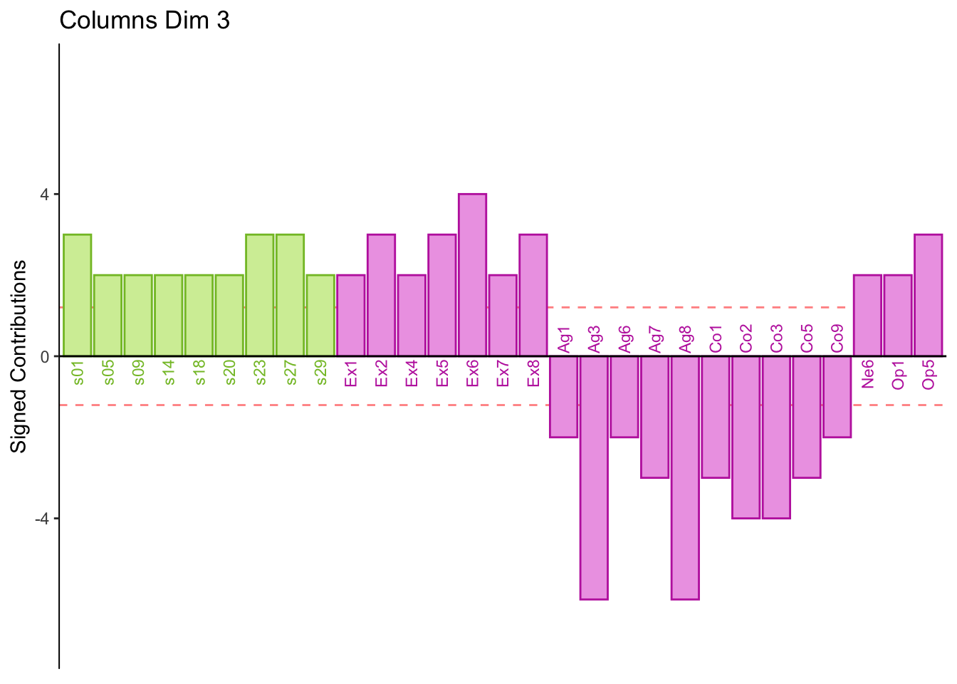
Dimension 3: Spatial, extroversion, openness (+) vs. consciousness, aggreeableness, object
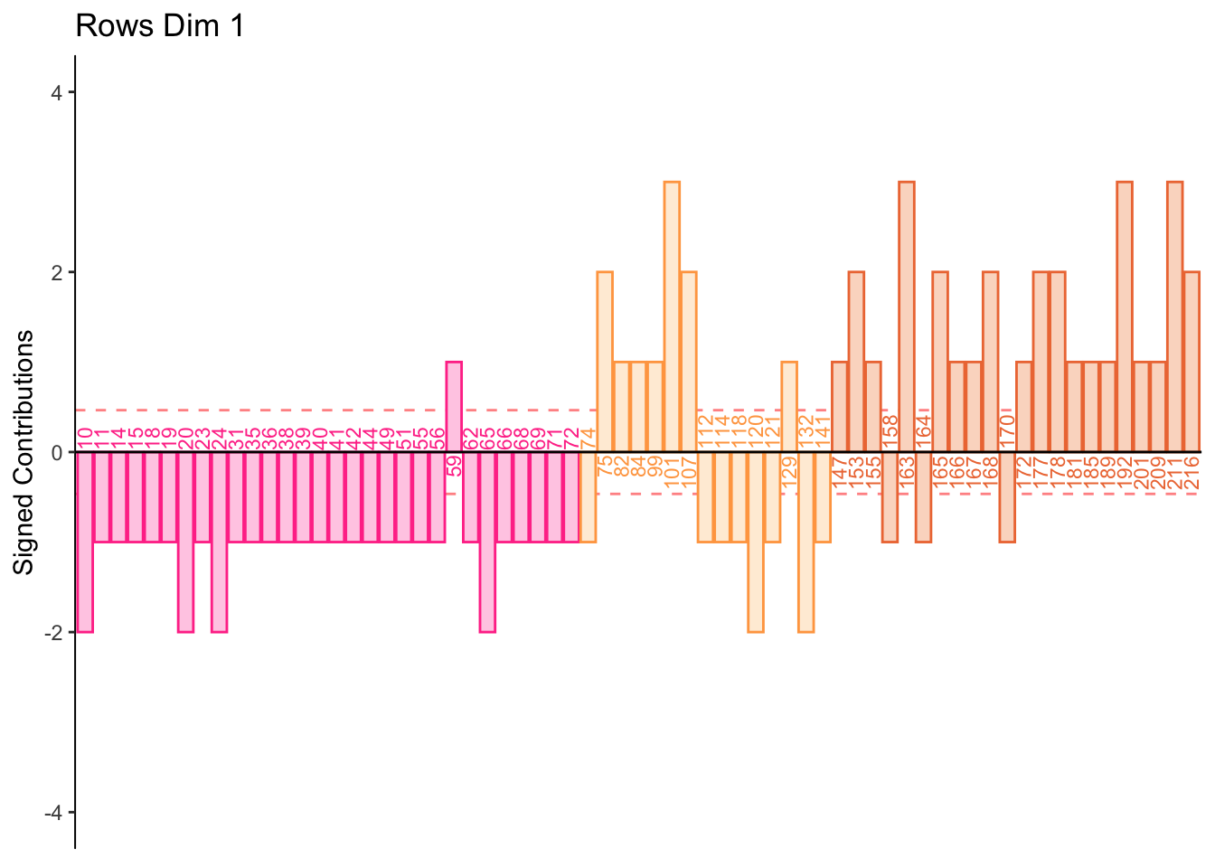
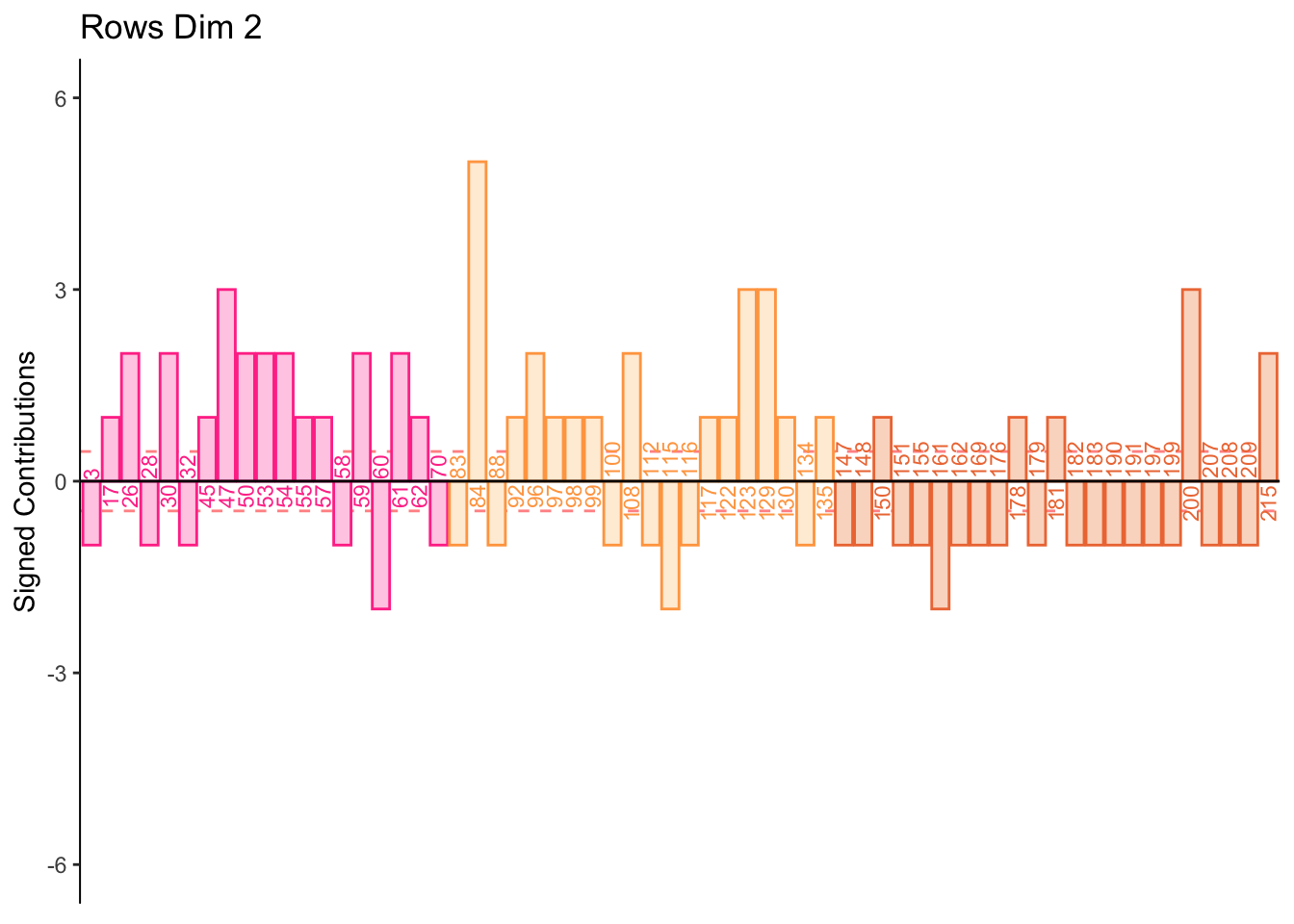
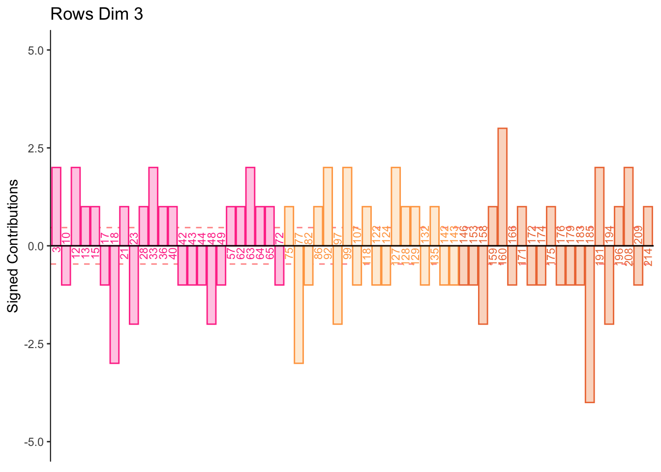
7.2.7 Contributions for Rows
7.2.8 Contributions for Columns
7.3 Summary
From the row and column contribution plots we can interpret (look for new information per dimension):
Dimension 1:
Half normal and all low memory groups score higher on PHQ and Neuroticism 1 i.e. “Can be cold and aloof”
Half normal and all high memory groups score higher on object, extroversion, and openness
Dimension 2:
Low memory scores higher on spatial
Dimension 3:
Some participants score higher on agreeableness and conscientiousness or visa versa