Chapter 8 DiSTATIS
In a sorting task the data collected will be collected in a matrix with the items in the rows and the groups in the columns called the indicator matrix for one judge. If the item is put into a group, then a 1 needs to marked in that column and 0’s in all the others.
The co-occurance matrix can be obtained by multiplying the indicator matrix by the transpose of itself creating an item by item matrix. If there is a 1 where the row and column intersects then that means those items were sorted together.
The distance matrix is computed by subtracting the co-occurance matrix from 1. If there is a 0 where the row and column intersects then that means those items were sorted together.
The cross-product matrix is computed by multi-dimensional scaling. Each element of the distance matrix is subtracted by the row and column mean, then added to the grand mean of the distance matrix, and then multiplied by negative one half.
The Rv coefficient between two different cross-product matrices (CP’s) are obtained by taking:
trace(t(CP1)CP2)/sqrt(trace(t(CP1)CP2)*trace(t(CP2)CP1)))A value of 1 means that the two assessors sorted the items identically and a 0 means they sorted completely different. They are then complied into a similartiy matrix where the number of rows and columns equals the number of assessors.
The weights for each judge (table) are obtained by the square root of each element (each element corresponds to each different table similarity) of the eigen vector obtained by the eigendecomposition (PCA) of the Rv matrix. Lower weights are associated with outliers and higher weights are associated with more homogeneous tables.
The compromise is computed by the sum of multiplying each judge’s cross-product matrix by its associated weight. Finally, a PCA is run on this compromise.
8.1 Data set: Beer Distance Matrix
The rows are 30 different beers sorted by 51 participants into 10 different groups. Each element of the table is which group the judge sorted the beer into. The design variables used will be gender or type of beers they consume (industrial vs. crafted).
| C1 | C2 | C3 | C4 | C5 | C6 | C7 | C8 | C9 | C10 | C11 | C12 | C13 | C14 | C15 | C16 | C17 | C18 | C19 | C20 | C21 | C22 | C23 | C24 | C25 | C26 | C27 | C28 | C29 | C30 | C31 | C32 | C33 | C34 | C35 | C36 | C37 | C38 | C39 | C40 | C41 | C42 | C43 | C44 | C45 | C46 | C47 | C48 | C49 | C50 | C51 | |
|---|---|---|---|---|---|---|---|---|---|---|---|---|---|---|---|---|---|---|---|---|---|---|---|---|---|---|---|---|---|---|---|---|---|---|---|---|---|---|---|---|---|---|---|---|---|---|---|---|---|---|---|
| Minerva PA | 1 | 1 | 1 | 1 | 1 | 1 | 1 | 1 | 1 | 1 | 1 | 1 | 1 | 1 | 1 | 1 | 1 | 1 | 1 | 1 | 1 | 1 | 1 | 1 | 1 | 1 | 1 | 1 | 1 | 1 | 1 | 1 | 1 | 1 | 1 | 1 | 1 | 1 | 1 | 1 | 1 | 1 | 1 | 1 | 1 | 1 | 1 | 1 | 1 | 1 | 1 |
| Cucapa Miel | 2 | 1 | 2 | 1 | 2 | 1 | 1 | 1 | 2 | 1 | 2 | 2 | 1 | 1 | 1 | 2 | 2 | 2 | 2 | 1 | 1 | 1 | 2 | 1 | 1 | 1 | 1 | 1 | 2 | 1 | 2 | 2 | 1 | 1 | 1 | 1 | 1 | 1 | 1 | 2 | 1 | 2 | 1 | 2 | 2 | 2 | 1 | 2 | 1 | 1 | 2 |
| Tempus Clasica | 2 | 1 | 3 | 1 | 2 | 1 | 1 | 2 | 2 | 2 | 1 | 2 | 1 | 1 | 1 | 1 | 1 | 1 | 1 | 1 | 1 | 2 | 1 | 1 | 1 | 1 | 1 | 2 | 1 | 1 | 1 | 1 | 2 | 1 | 2 | 1 | 1 | 1 | 2 | 1 | 2 | 3 | 1 | 2 | 1 | 1 | 2 | 2 | 2 | 2 | 1 |
| Tempus DM | 3 | 1 | 3 | 1 | 2 | 1 | 1 | 2 | 2 | 2 | 1 | 2 | 1 | 2 | 1 | 1 | 2 | 1 | 3 | 1 | 1 | 3 | 2 | 1 | 1 | 2 | 1 | 2 | 1 | 1 | 3 | 1 | 2 | 1 | 2 | 1 | 1 | 1 | 2 | 3 | 2 | 4 | 1 | 2 | 1 | 1 | 1 | 3 | 2 | 2 | 1 |
| Calavera MIS | 4 | 1 | 2 | 1 | 2 | 1 | 2 | 1 | 2 | 2 | 1 | 2 | 2 | 1 | 1 | 1 | 1 | 1 | 4 | 2 | 1 | 1 | 2 | 1 | 1 | 1 | 1 | 1 | 1 | 1 | 1 | 1 | 1 | 1 | 1 | 1 | 1 | 1 | 1 | 3 | 2 | 2 | 2 | 1 | 2 | 3 | 1 | 4 | 1 | 3 | 2 |
| Minerva Stout | 4 | 1 | 1 | 1 | 1 | 1 | 1 | 1 | 1 | 1 | 1 | 2 | 1 | 1 | 1 | 1 | 1 | 1 | 1 | 1 | 1 | 3 | 1 | 1 | 1 | 2 | 1 | 2 | 1 | 1 | 1 | 3 | 1 | 1 | 1 | 1 | 1 | 1 | 1 | 3 | 1 | 4 | 1 | 1 | 1 | 1 | 1 | 1 | 1 | 4 | 1 |
8.2 Analysis
8.2.1 Correlation Plot
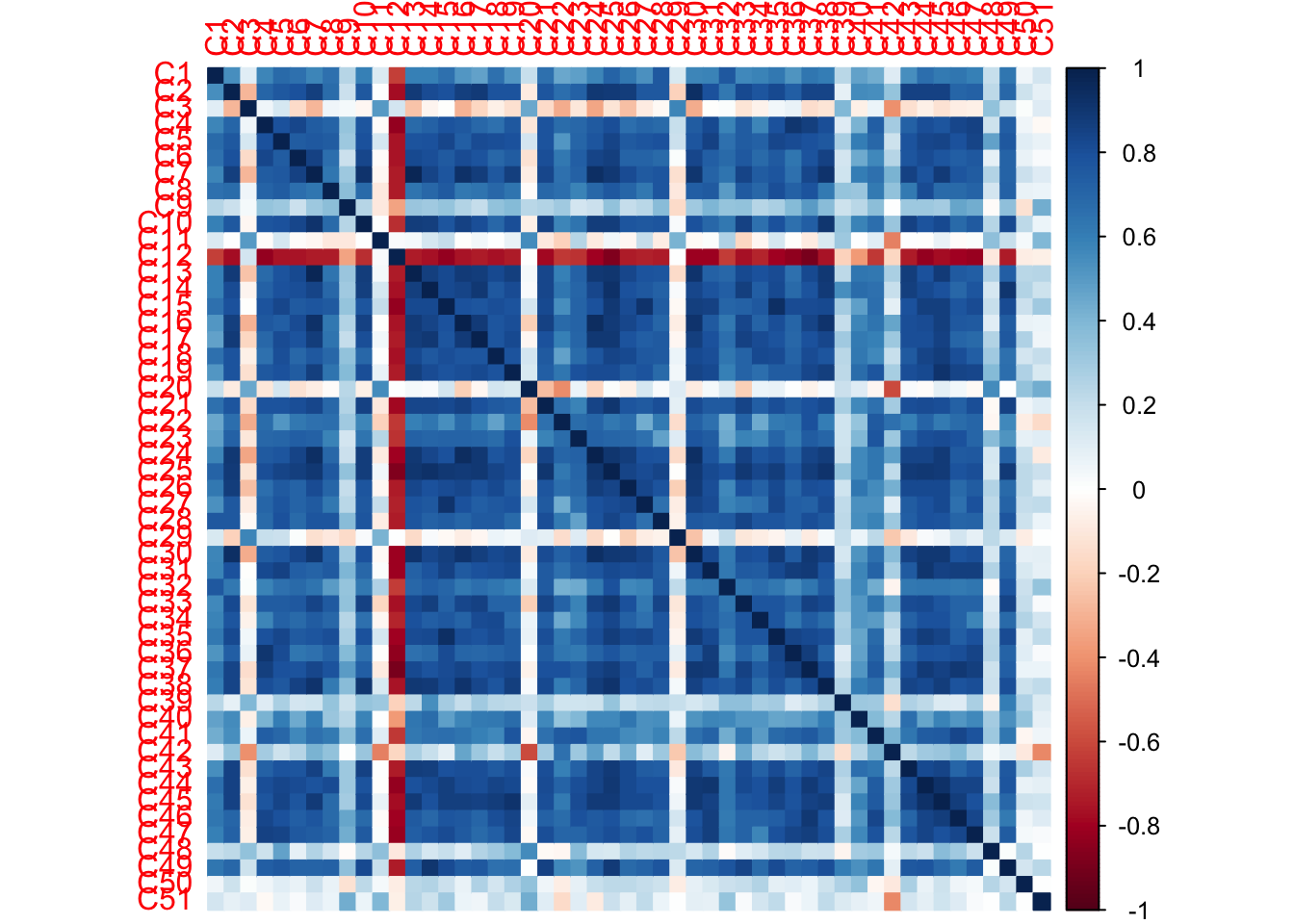
From the correlation table of the raw data set the 12th judge is negatively correlating with all other judges besides 3rd, 11th, 20th, 29th, 39th, 42nd, 48th, 50th, and 51st (these judges show a very low overall correlation with all participants).
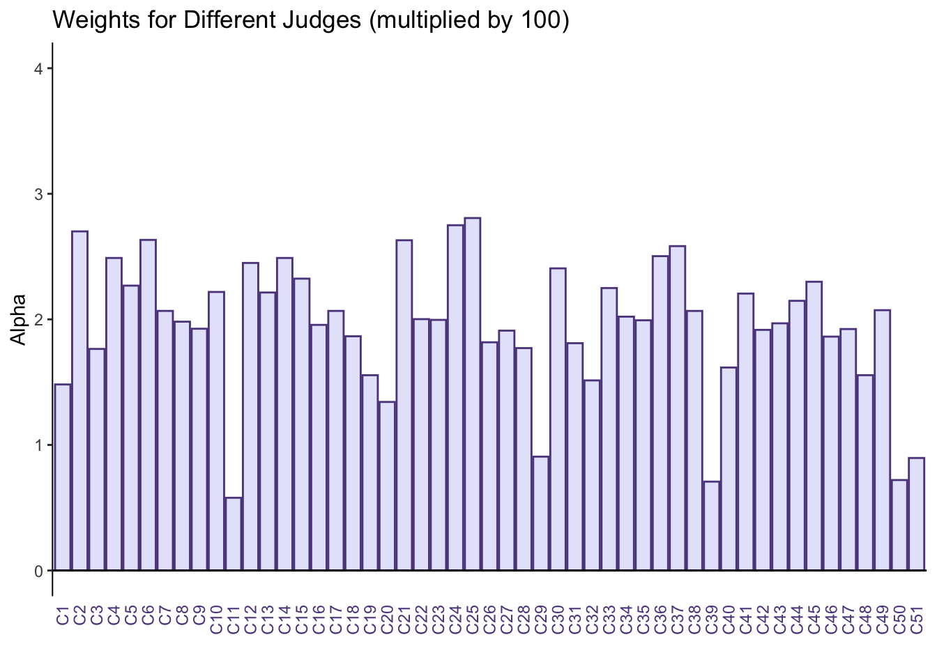
8.2.2 RV Matrix Correlation and Weights for Each Table
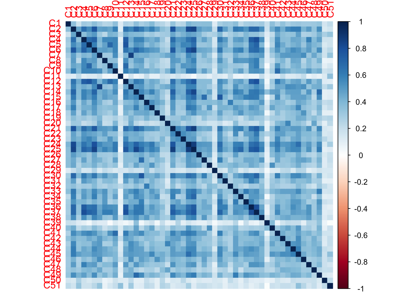
The Rv matrix correlation plot shows that all tables are positively correlated with each other i.e. each judge is their own table.
From the weights we can see taht judge 11, 29, 39, 50, and 51 sort the beers very differently from the rest of the judges.
8.2.3 Scree Plot
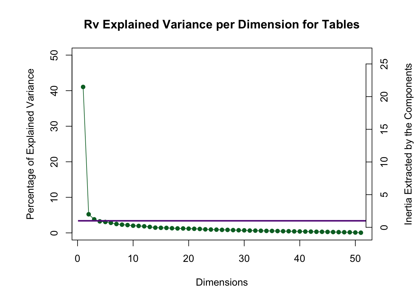
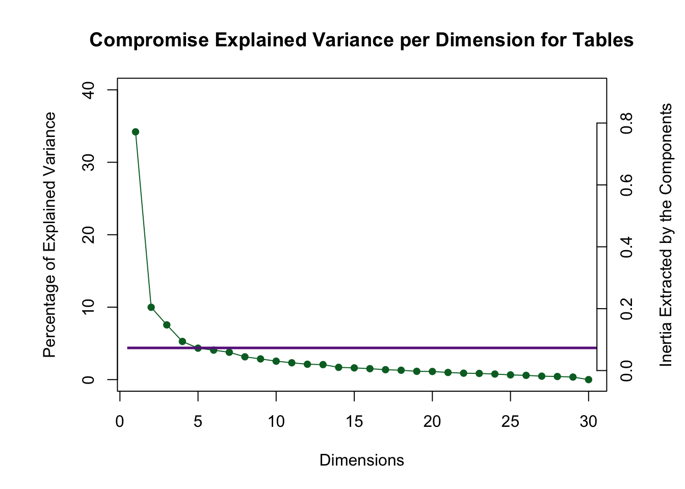
The Rv scree plot shows that the first two dimensions are above the Kaiser line and since there is such a large first dimension this is a signal that the judges are homogenous.
The compromise scree plot shows that the first four dimensions are above the Kaiser line. This is how we determine how many dimensions will be analyzed.
8.2.4 Rv Loadings
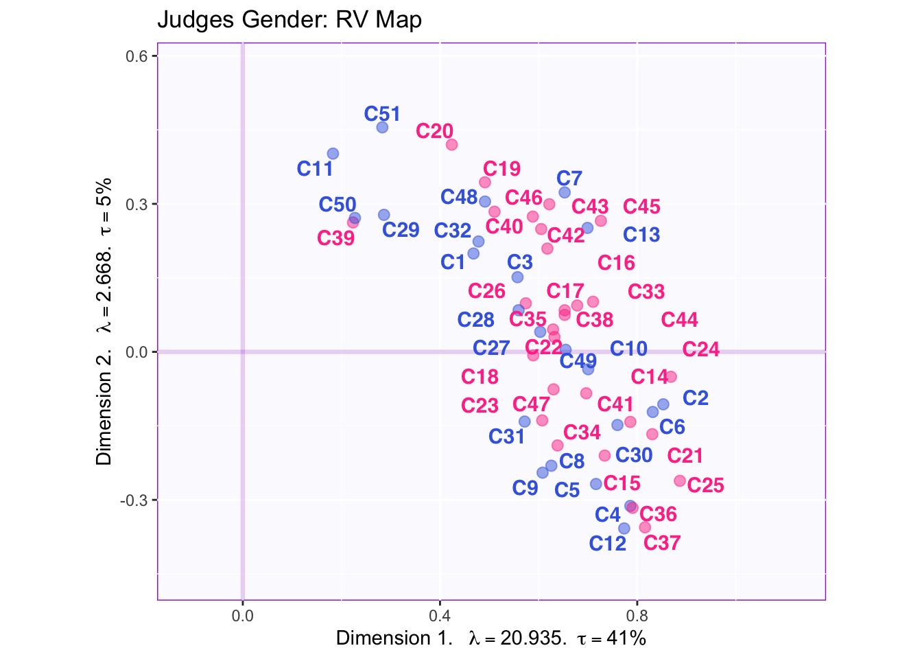
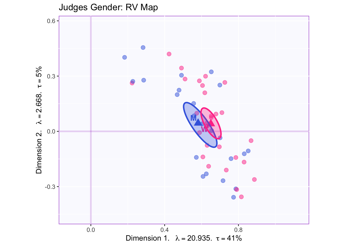
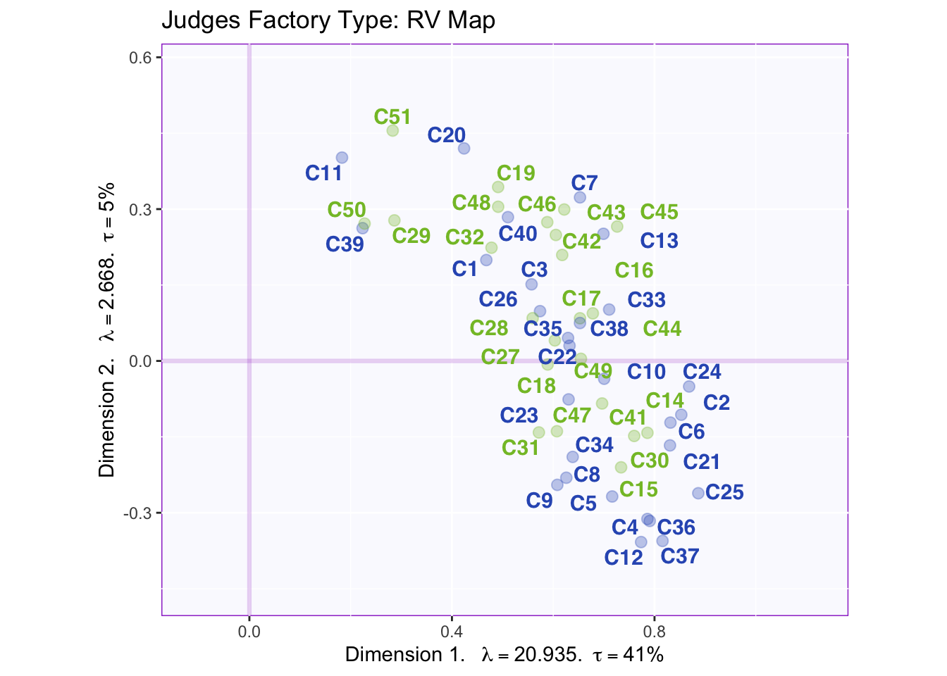
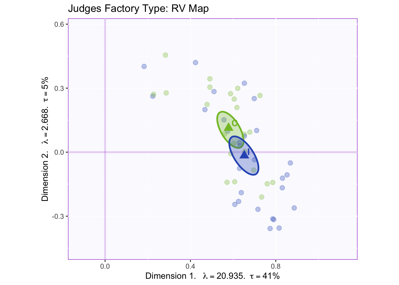
The RV maps of both design variables show that there is not a reliable difference between gender or what type of beer they consume.
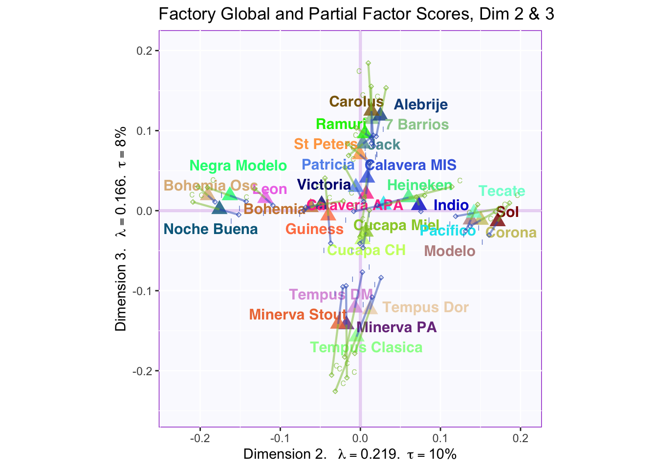
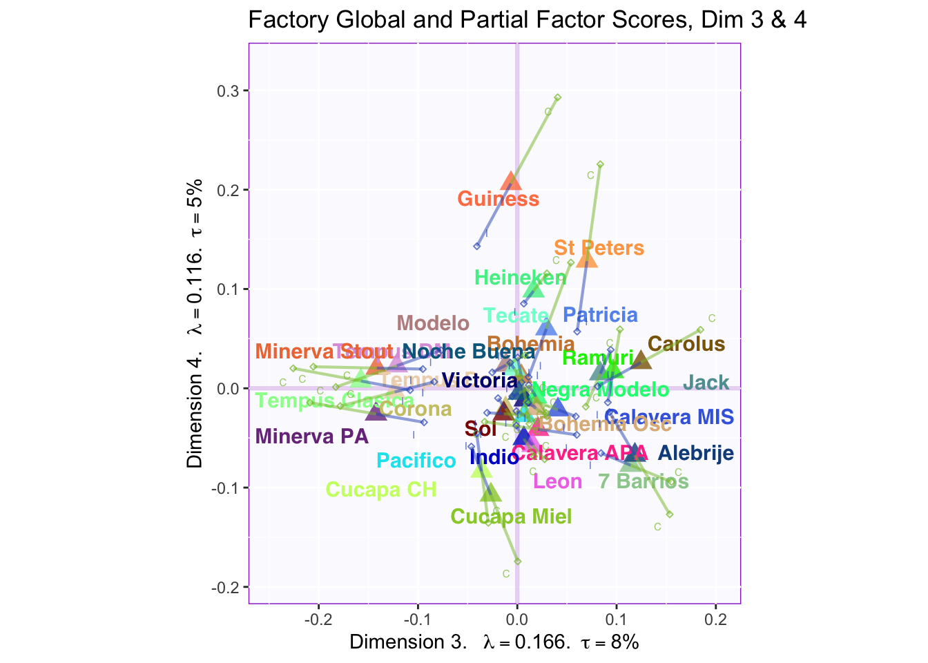
8.2.5 Global Factor Scores with Partial Factor Scores
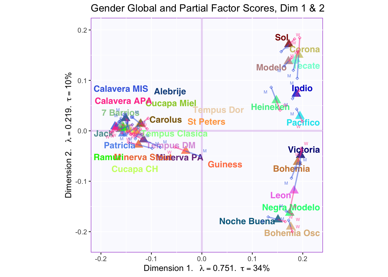
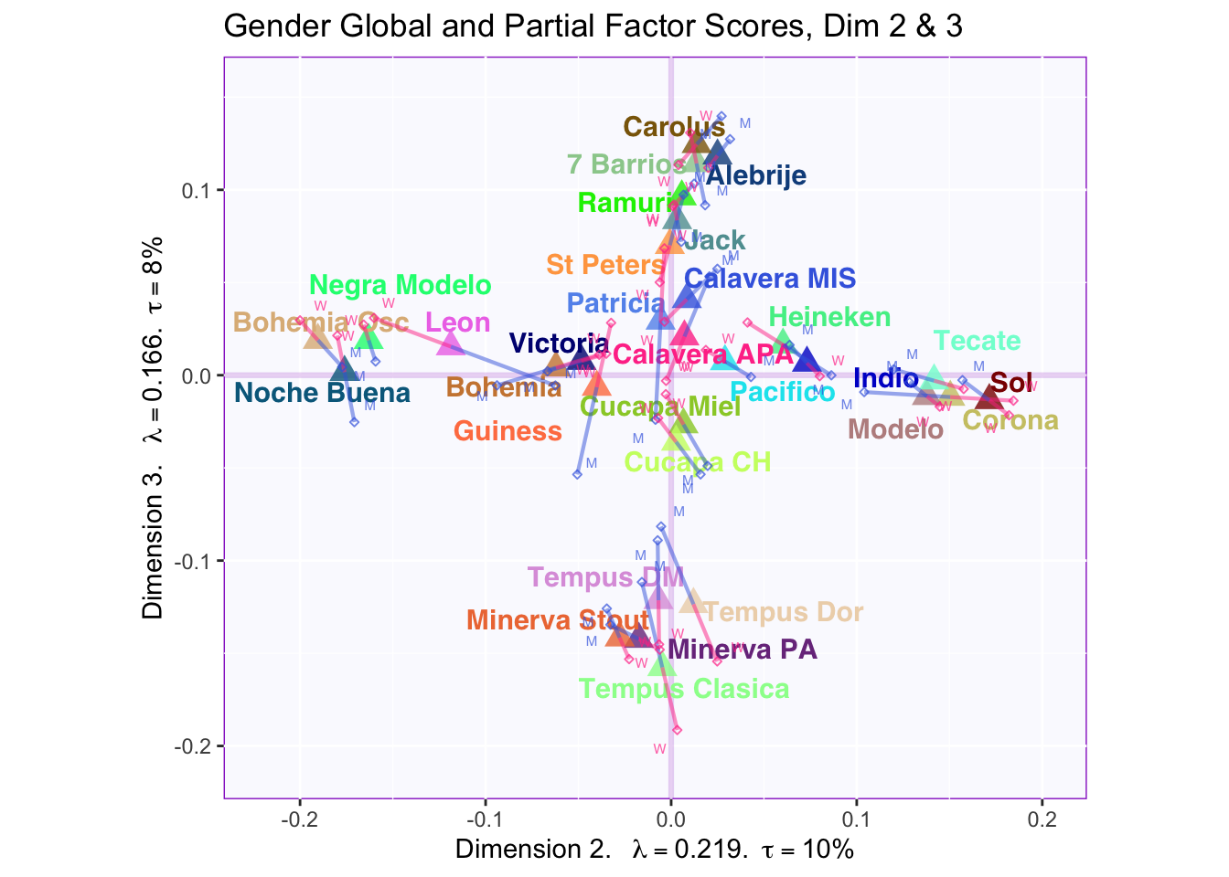
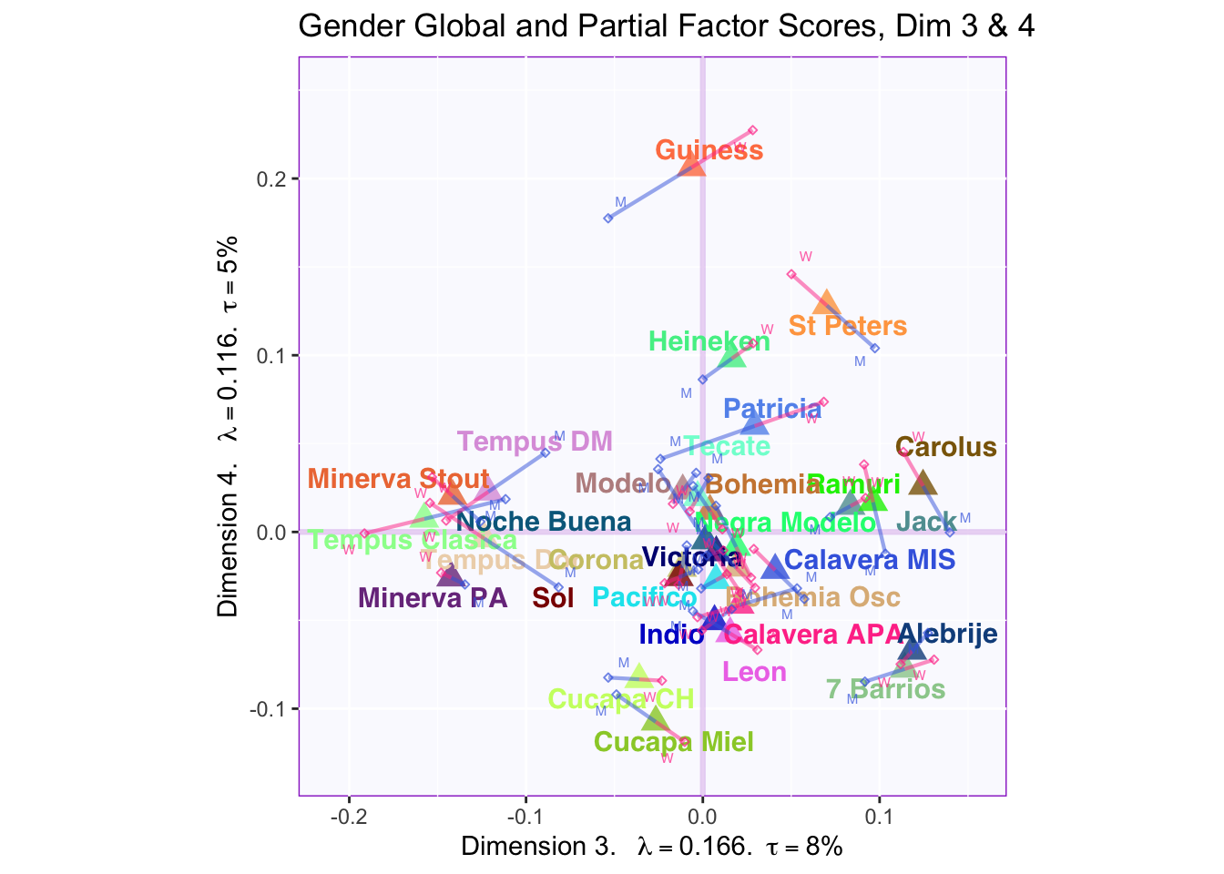
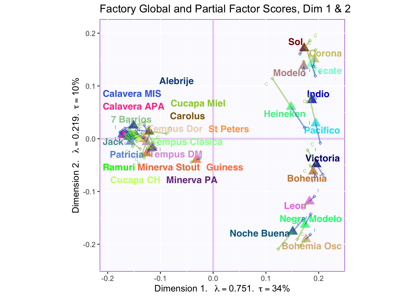
These plots are a bit messy, but from first appearnaces in the gender global and partial factor scores it looks as if men and women seem to be explaining similar amounts of variance.
However, in the types of beer they consume crafted beer is explaining more variance than industrial beer.
8.2.6 K-means to determine beer grouping and Cluster Analysis
#Suggests number of optimal clusters (data driven)
Centroids <- NbClust(resDiSTATIS$res4Splus$F, method = "kmeans", index = "alllong")
## Warning in pf(beale, pp, df2): NaNs produced
## Warning in pf(beale, pp, df2): NaNs produced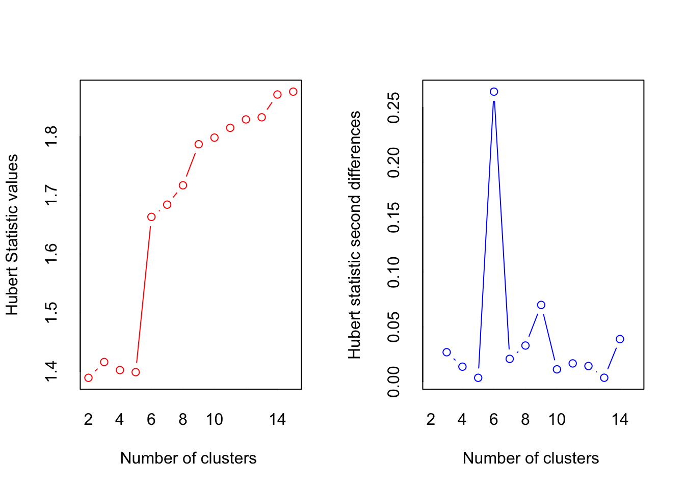
## *** : The Hubert index is a graphical method of determining the number of clusters.
##                 In the plot of Hubert index, we seek a significant knee that corresponds to a
##                 significant increase of the value of the measure i.e the significant peak in Hubert
##                 index second differences plot.
## 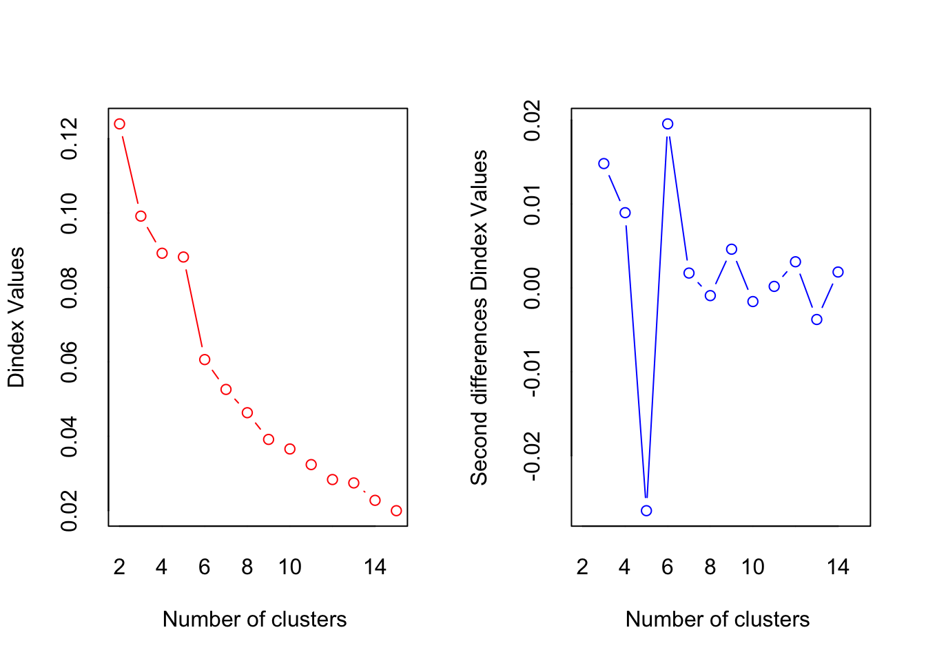
## *** : The D index is a graphical method of determining the number of clusters.
##                 In the plot of D index, we seek a significant knee (the significant peak in Dindex
##                 second differences plot) that corresponds to a significant increase of the value of
##                 the measure.
##
## *******************************************************************
## * Among all indices:
## * 8 proposed 2 as the best number of clusters
## * 5 proposed 3 as the best number of clusters
## * 1 proposed 4 as the best number of clusters
## * 1 proposed 5 as the best number of clusters
## * 3 proposed 6 as the best number of clusters
## * 1 proposed 9 as the best number of clusters
## * 3 proposed 14 as the best number of clusters
## * 6 proposed 15 as the best number of clusters
##
##                    ***** Conclusion *****
##
## * According to the majority rule, the best number of clusters is  2
##
##
## *******************************************************************
#suggested is 2 clusters, but need four to see separation on significant dimensions above kiaser line
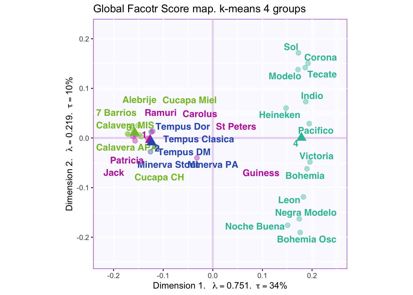
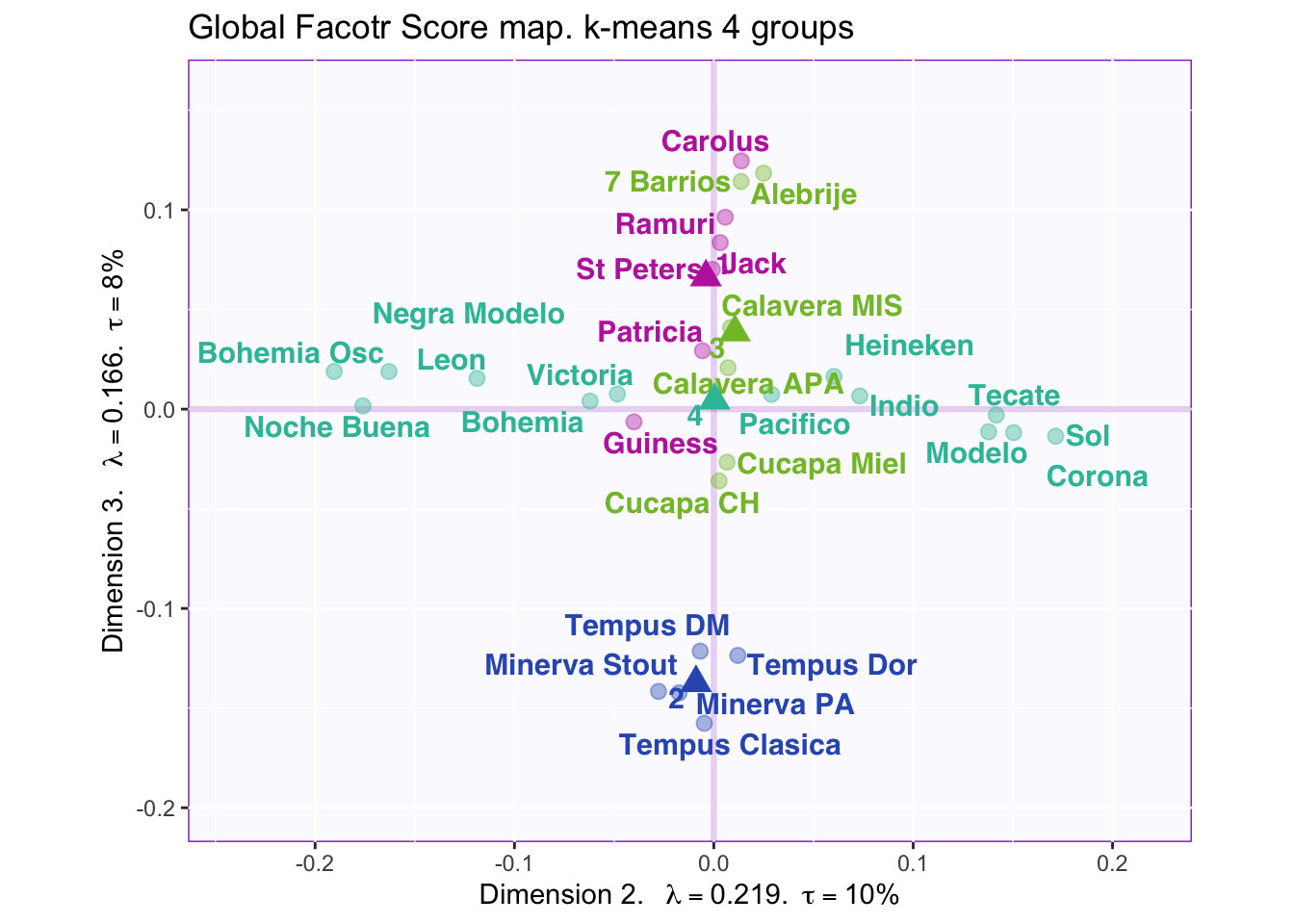
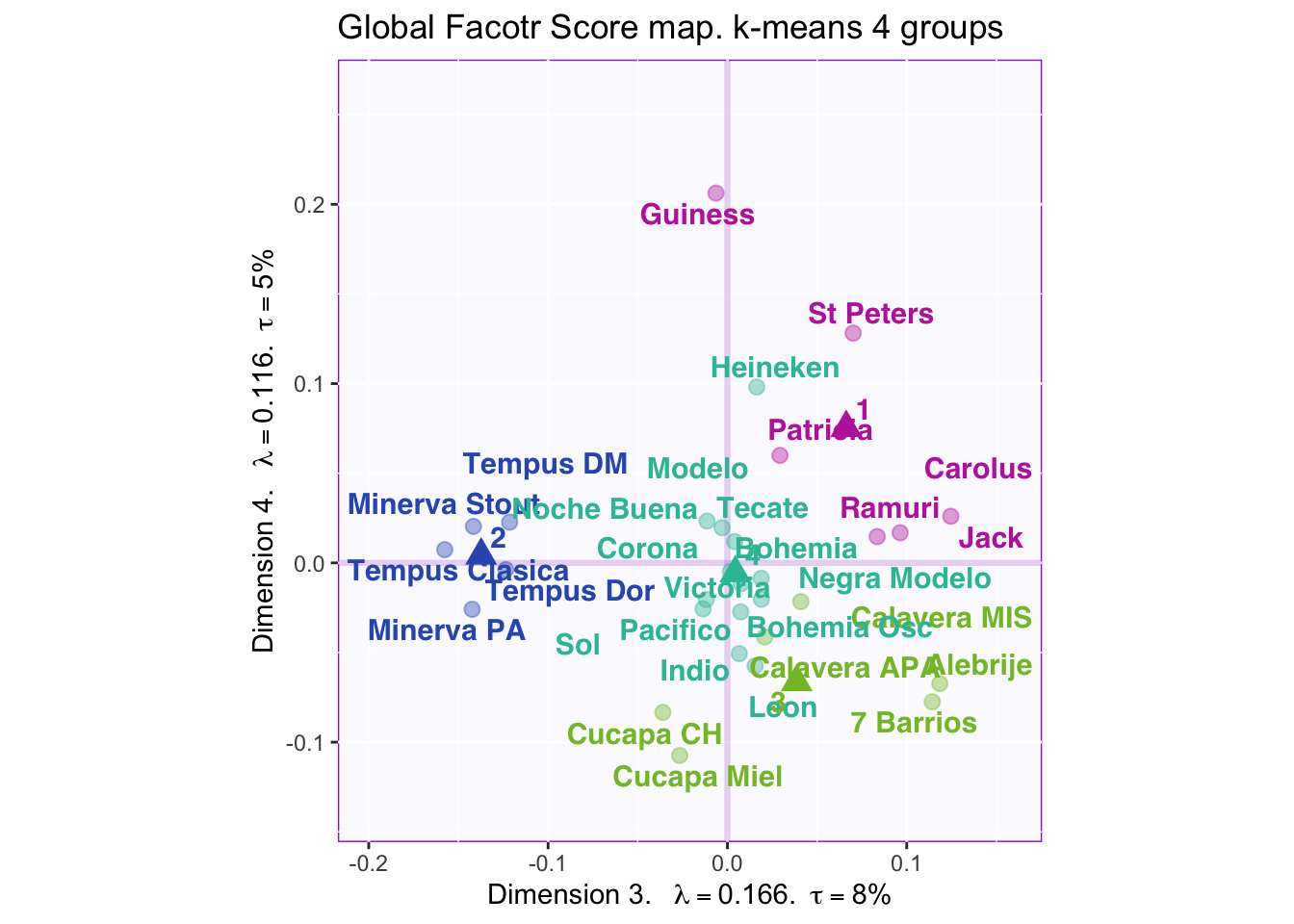
beer.kmeans <- kmeans(resDiSTATIS$res4Splus$F, centers = 4)
#rownames(beer.kmeans$centers) <- c("A.S.I","Lager")
#Plot with centroids and beers
col4Clusters <- createColorVectorsByDesign(makeNominalData(as.data.frame(beer.kmeans$cluster)))
# A tweak for colors
in.tmp <- sort(rownames(col4Clusters$gc), index.return = TRUE)$ix
col4Centroids <- col4Clusters$gc[in.tmp]
#
for (k in 1:3) {
baseMap.i.km <- PTCA4CATA::createFactorMap(resDiSTATIS$res4Splus$F,
title = "Global Facotr Score map. k-means 4 groups",
axis1 = k, axis2 = k+1,
col.points = col4Clusters$oc,
col.labels = col4Clusters$oc,
alpha.points = .4)
centroidmap <- PTCA4CATA::createFactorMap(beer.kmeans$centers,
axis1 = k, axis2 = k+1,
col.points = col4Centroids,
col.labels = col4Centroids,
cex = 4,
pch = 17,
alpha.points = 1)
fi.labels <- createxyLabels.gen(k, k+1,
lambda = resDiSTATIS$res4Splus$eigValues,
tau = resDiSTATIS$res4Splus$tau,
axisName = "Dimension ")
a06.aggMap.i.km <- baseMap.i.km$zeMap_background +
baseMap.i.km$zeMap_dots + baseMap.i.km$zeMap_text + fi.labels + centroidmap$zeMap_dots + centroidmap$zeMap_text
print(a06.aggMap.i.km)
}
####################################################################################
#Cluster Analysis
D4Prod <- dist(resDiSTATIS$res4Splus$F, method = "euclidean")
fit4Prod <- hclust(D4Prod, method = "ward.D2")
b3.tree4Product <- fviz_dend(fit4Prod, k = 1,
k_colors = 'burlywood4',
label_cols = col4Clusters$oc, cex = .7, xlab = 'Beers',
main = 'Cluster Analysis: Beers')

print(b3.tree4Product)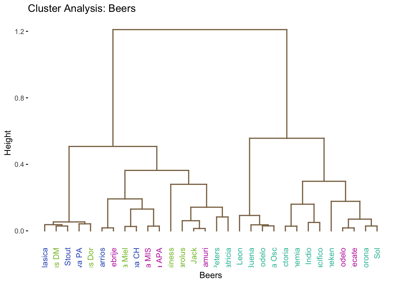
Kmeans:
Data driven way to find the centriod of each group. The first step is to randomly generate a desired number of centroids. Each data point is then assigned to a centroid based on squared Euclidean distance. Then the centroids are recomputed by taking the mean of all the data points assigned to the cluster. These steps continue to iterate until the centroids become stable. Be careful as the result may be a local minimum!!
According to the “knee test” of the supporting plots (Hubert statistic second difference and Second differences Dindex Values) it would support that 6 clusters would have the best “measure.” However, 6 clusters creates groups of only one or two beers so boostraping the confidence intervals is impossible. 7 centers finally shows the separation in the large group on the positive side of dimension 1, but this still has the same problem as 6 clusters. The reason 4 clusters were chosen to try to find separation in all four dimensions. The highest suggested number of clusters is 2, but they are only separated on the first dimension, which finds the overall effect (nothing really interesting here considering it is only separating ale, stout, and IPA (strong taste) into one group and more mild tasting beers into the other).
However, groups are not obviously defined with 4 clusters i.e. the beer types, locations where it was produced, alcohol content, and color are mixed within the groups.
Cluster Analysis:
See ?hclust for description:
“This function performs a hierarchical cluster analysis using a set of dissimilarities for the n objects being clustered. Initially, each object is assigned to its own cluster and then the algorithm proceeds iteratively, at each stage joining the two most similar clusters, continuing until there is just a single cluster. At each stage distances between clusters are recomputed by the Lance–Williams dissimilarity update formula according to the particular clustering method being used.”
The dissimilarity matrix is the euclidean distance (for this example) between the rows of the factor scores for the different beers.
Shows that possibly two or four groups could capture a difference between the groups.
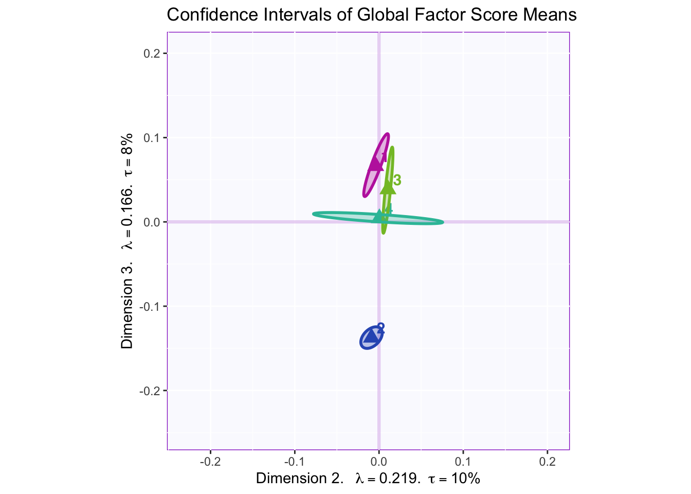
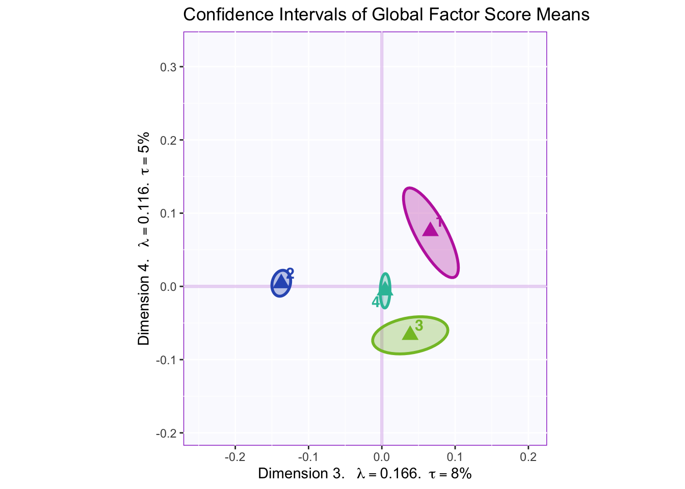
8.2.7 Confidence Intervals of Mean Global Factor Scores
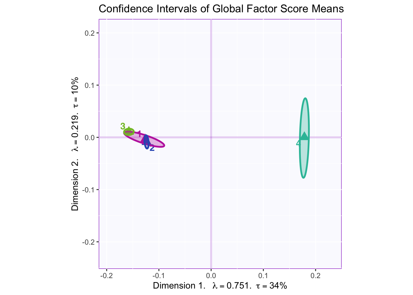
Dimension 1: 4 (+) vs. others (-)
Dimension 2: Hard to tell, but 1 and 2 (-) vs 3 (+)
Dimension 3: Others (+) vs. 2 (-)
Dimension 4: 1 and maybe 2 (+) vs 3 (-)
8.2.8 Mean Global and Partial Factor Scores
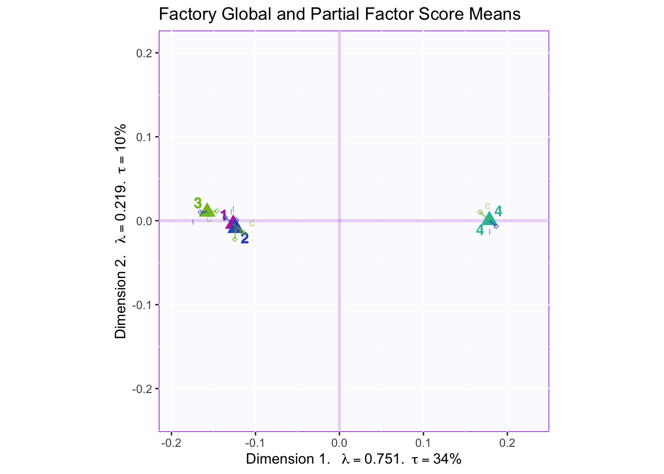
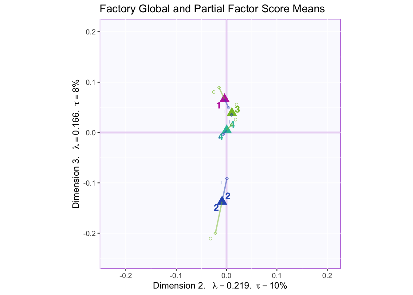
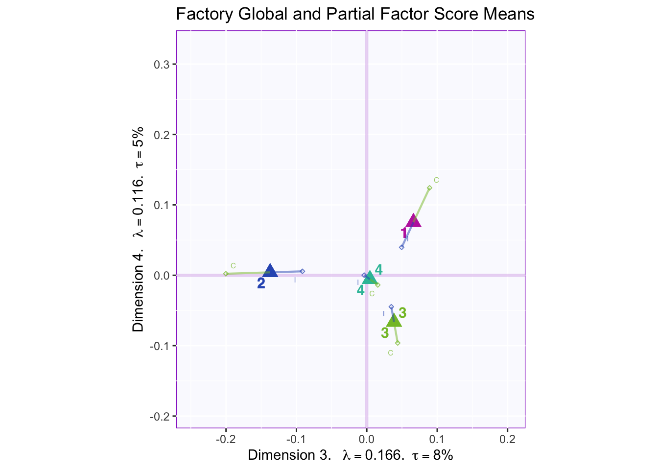
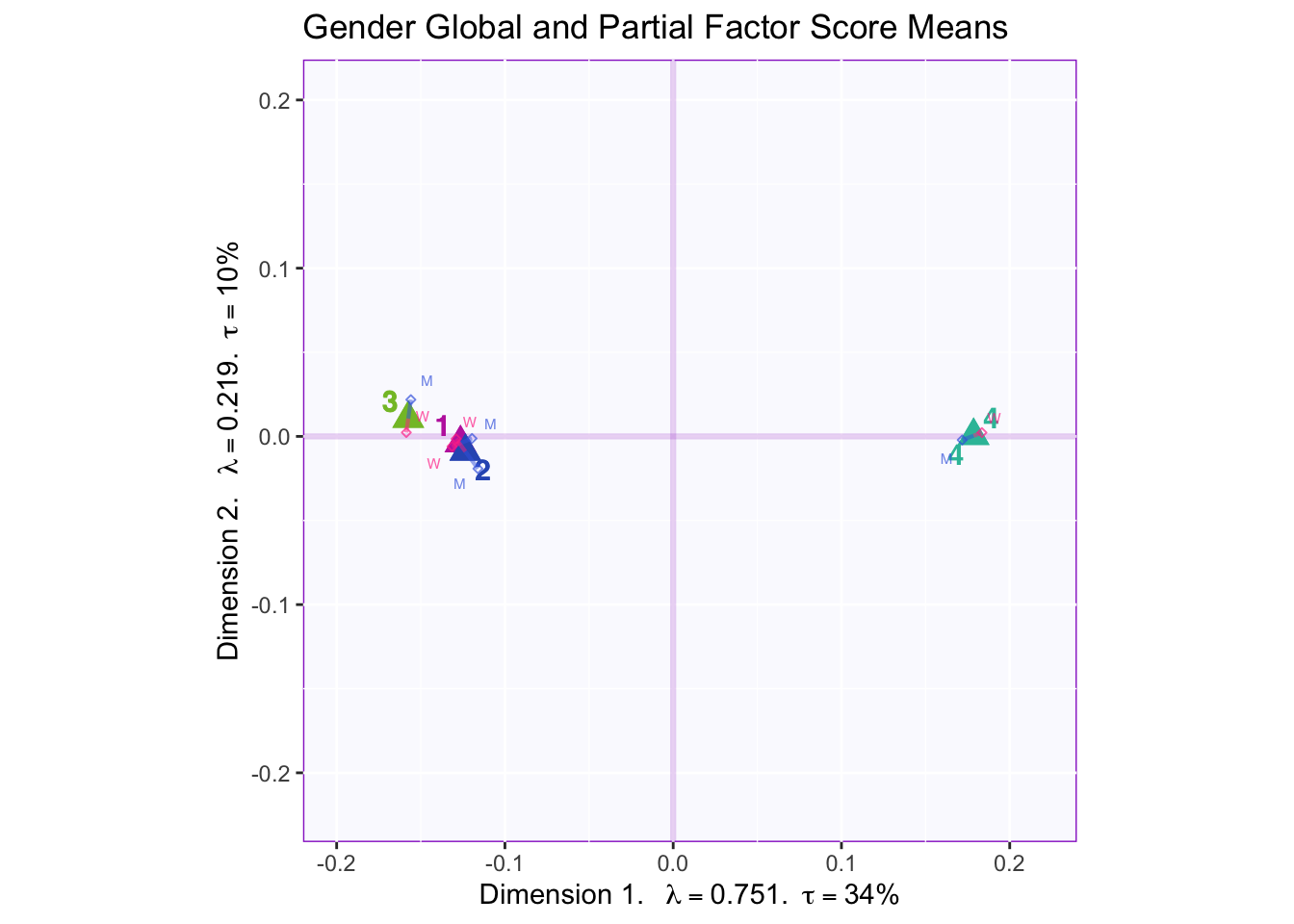
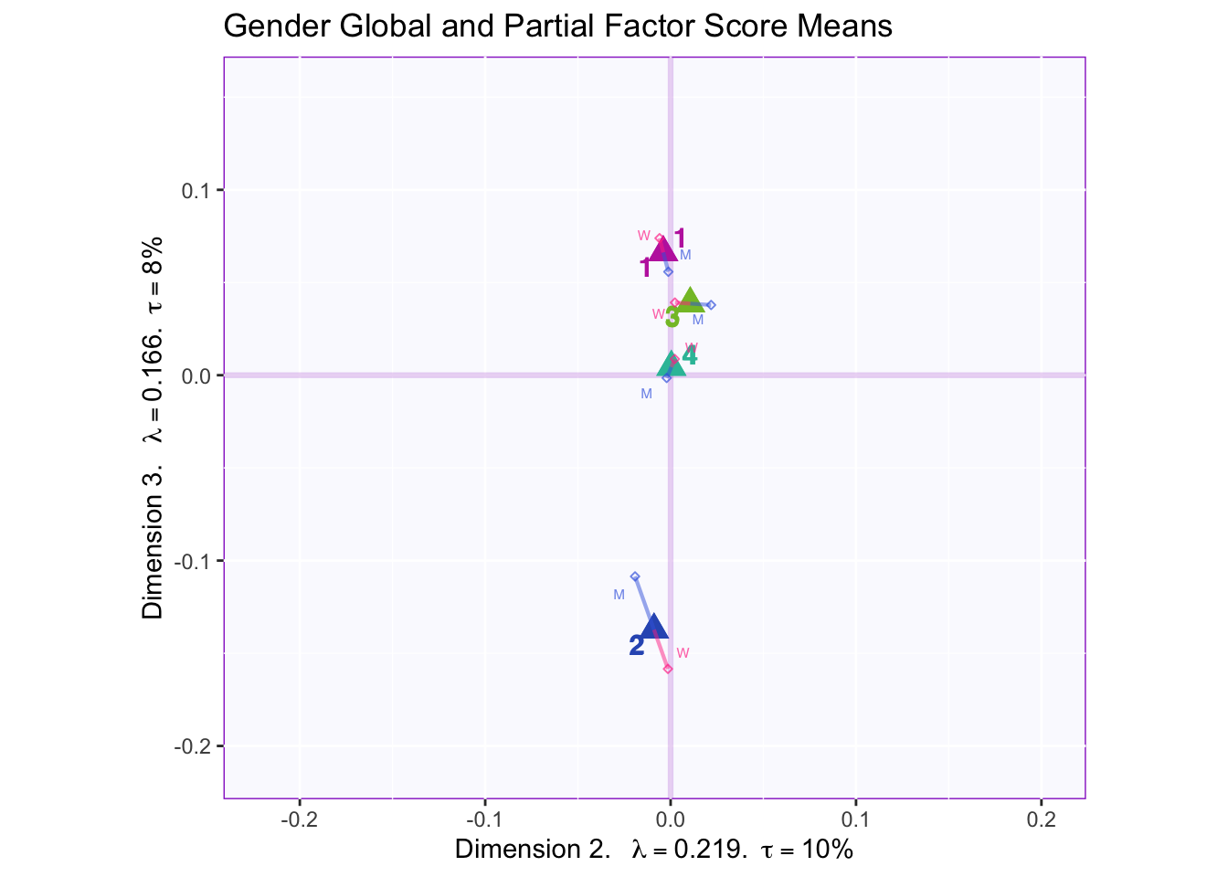
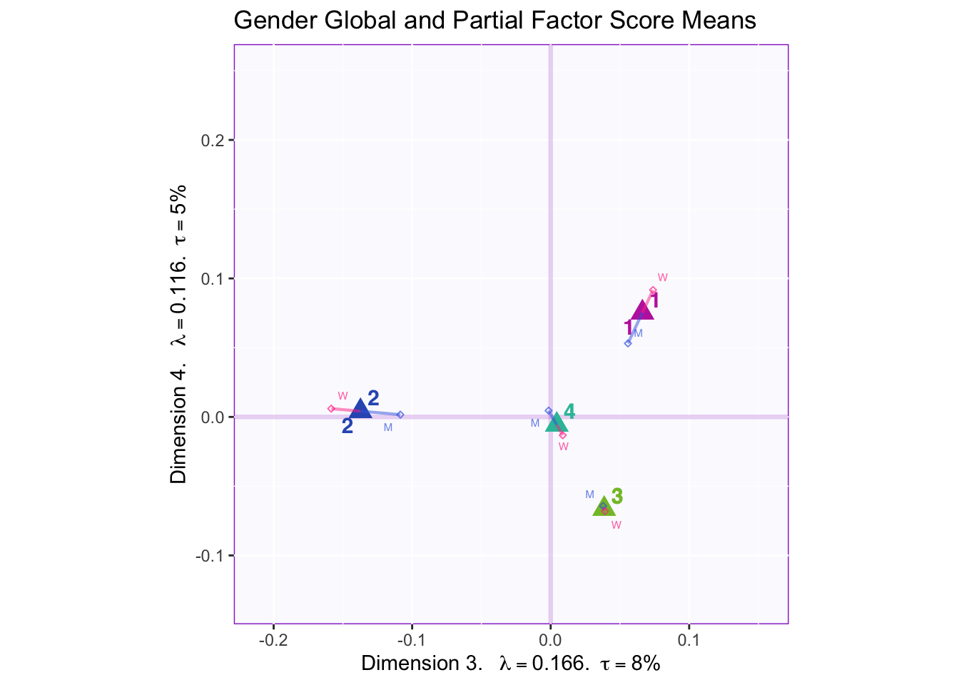
In both the gender and beer they consume plots groups 1 and 2 they have the biggest variance in dimensions 2 to 4. In the dimension 1 and 2 plots there isn’t much variance between the judges.
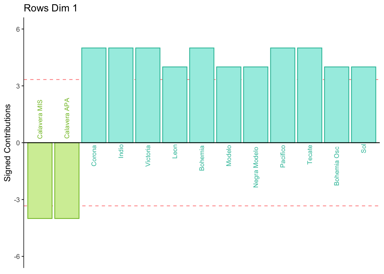
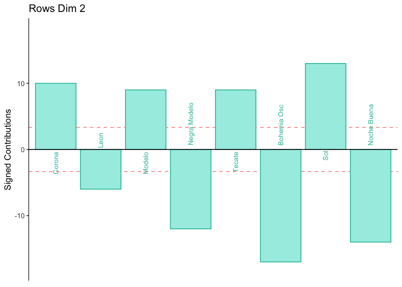
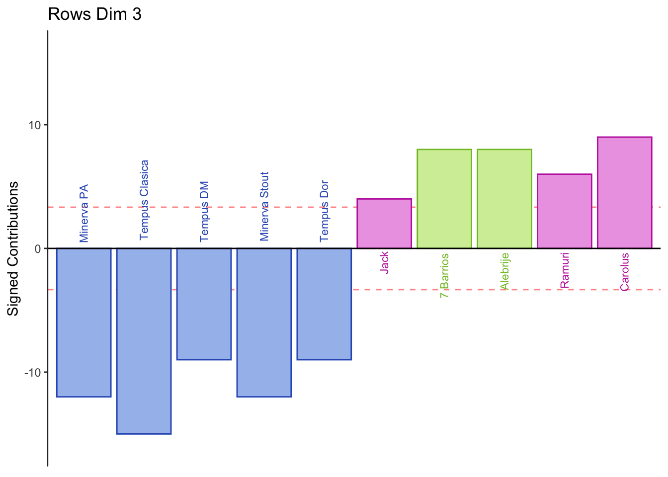
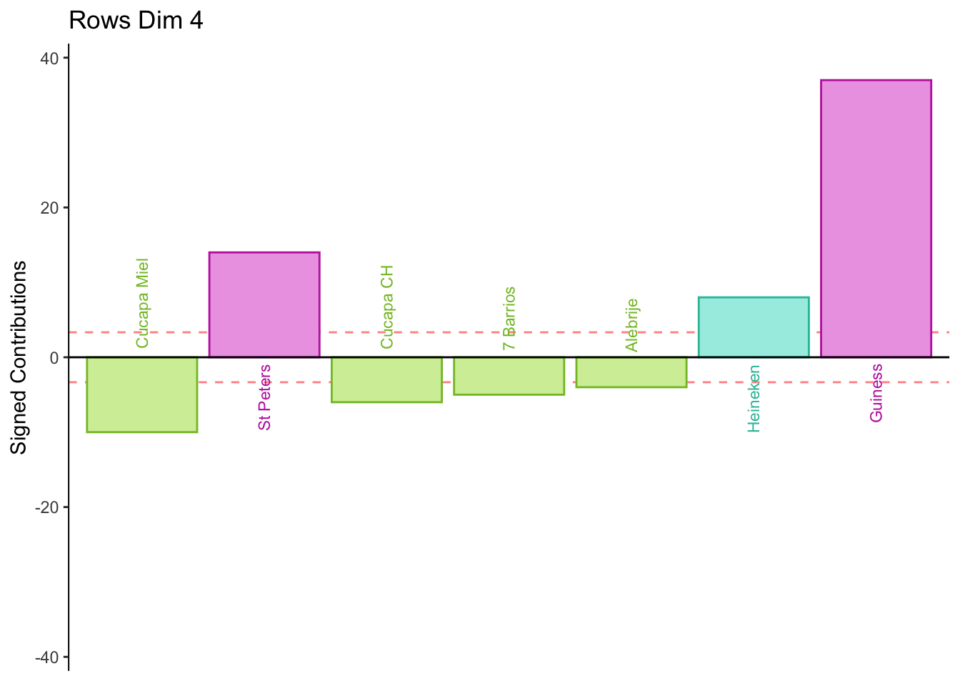
8.2.9 Contributions for Rows
Fj <- resDiSTATIS$res4Splus$F
F2 <- Fj**2
SF2 <- apply(F2, 2, sum)
ctrj <- t(t(F2)/SF2)
signed.ctrj <- ctrj * sign(Fj)
rownames(signed.ctrj) <- rownames(JollyFellow)

for (k in 1:4) {
c001.plotCtrj.1 <- PrettyBarPlot2(
                       bootratio = round(100*signed.ctrj[,k]),
                       signifOnly = TRUE,
                       threshold = 100 / nrow(signed.ctrj),
                       ylim = NULL,
                       color4bar = col4Clusters$oc,
                       color4ns = "gray75",
                       plotnames = TRUE,
                       main = paste('Rows Dim', k),
                       ylab = "Signed Contributions")
print(c001.plotCtrj.1)
#c001.plotCtrj.1 <- recordPlot()
}
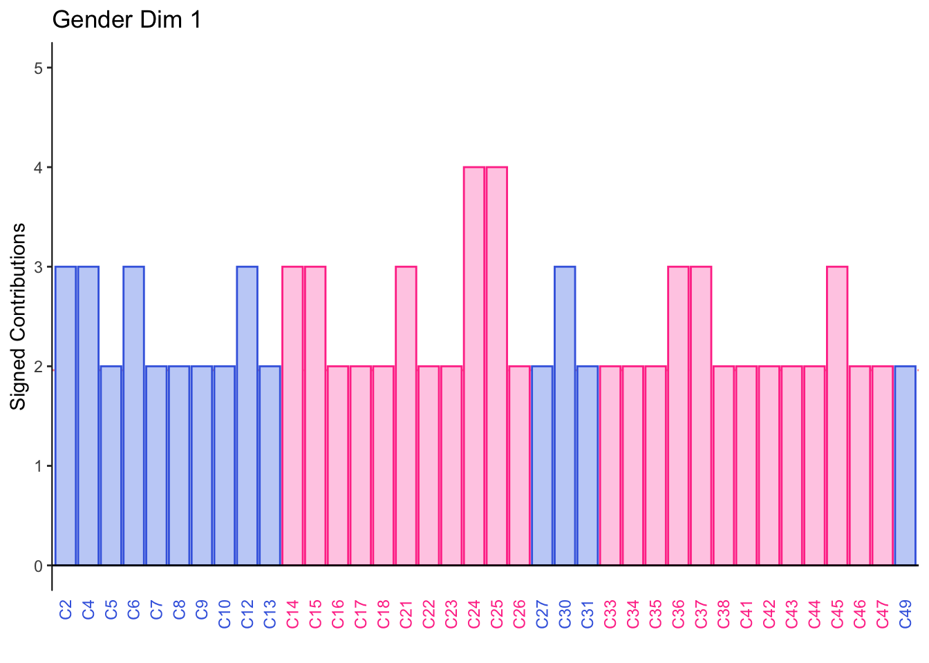
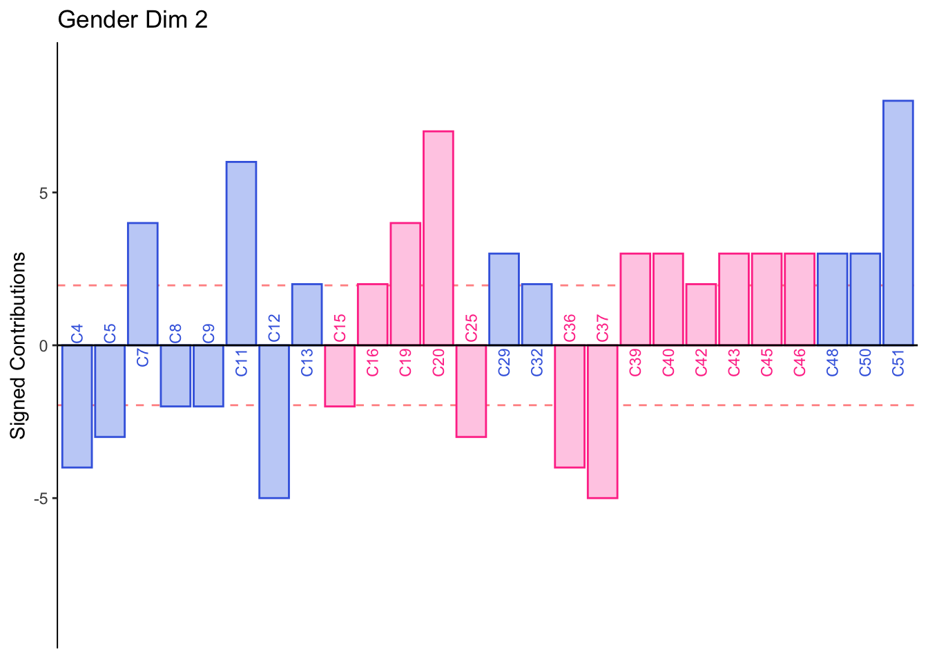
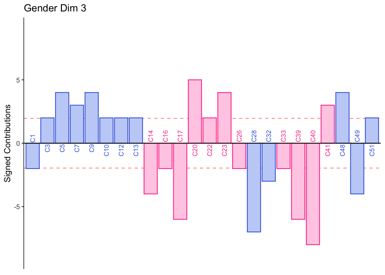
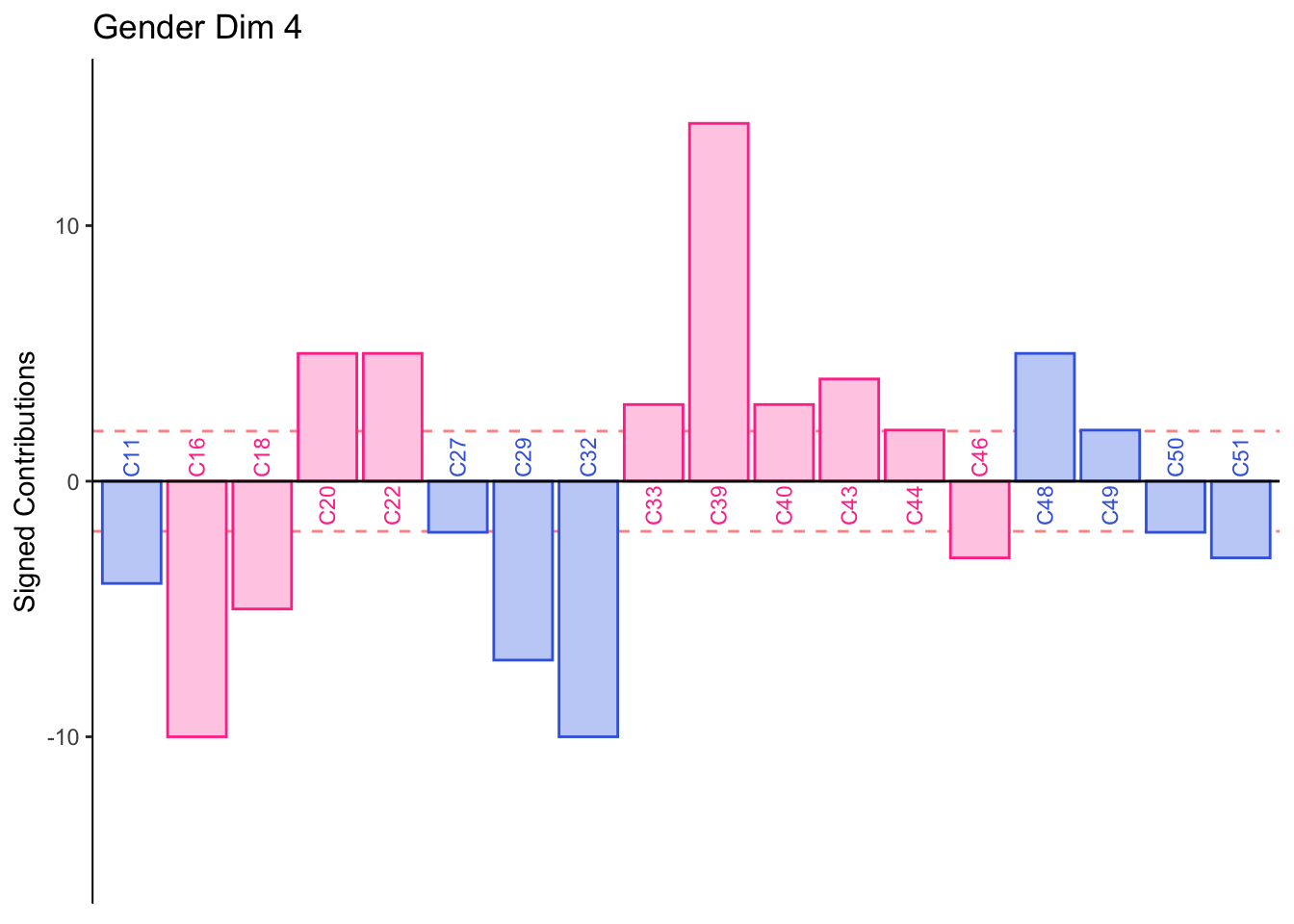
8.2.10 Contributions for Columns
Fj <- resDiSTATIS$res4Cmat$G
RvFS <- Fj**2
RvSF2 <- apply(RvFS, 2, sum)
ctrj <- t(t(RvFS)/RvSF2)
signed.ctrj <- ctrj * sign(Fj)

#Gender
for (k in 1:4) {
c001.plotCtrj.1 <- PrettyBarPlot2(
                       bootratio = round(100*signed.ctrj[,k]),
                       signifOnly = TRUE,
                       threshold = 100 / nrow(signed.ctrj),
                       ylim = NULL,
                       color4bar = color4Gender.list$oc,
                       color4ns = "gray75",
                       plotnames = TRUE,
                       main = paste('Gender Dim', k),
                       ylab = "Signed Contributions")
print(c001.plotCtrj.1)
#c001.plotCtrj.1 <- recordPlot()
}
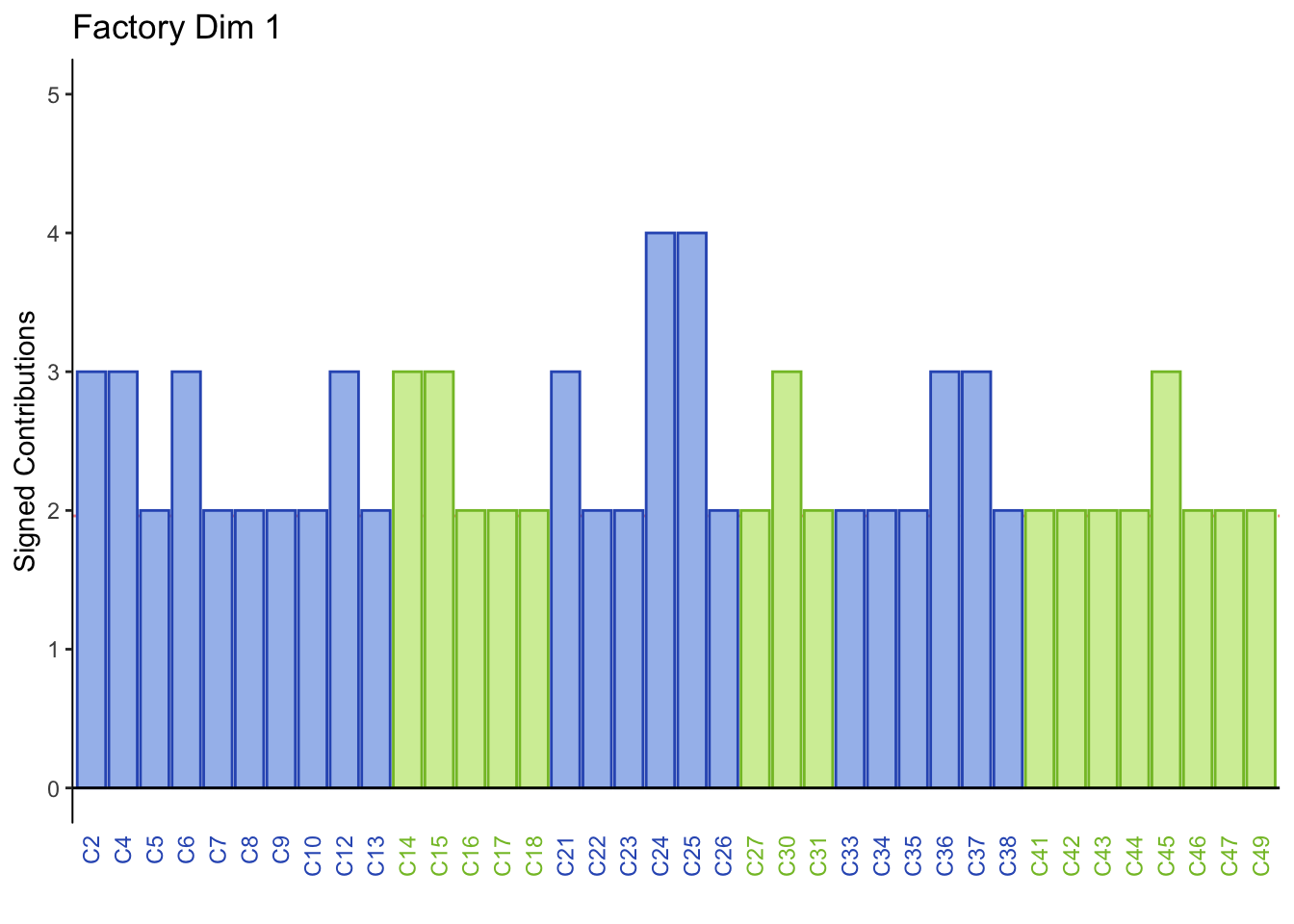
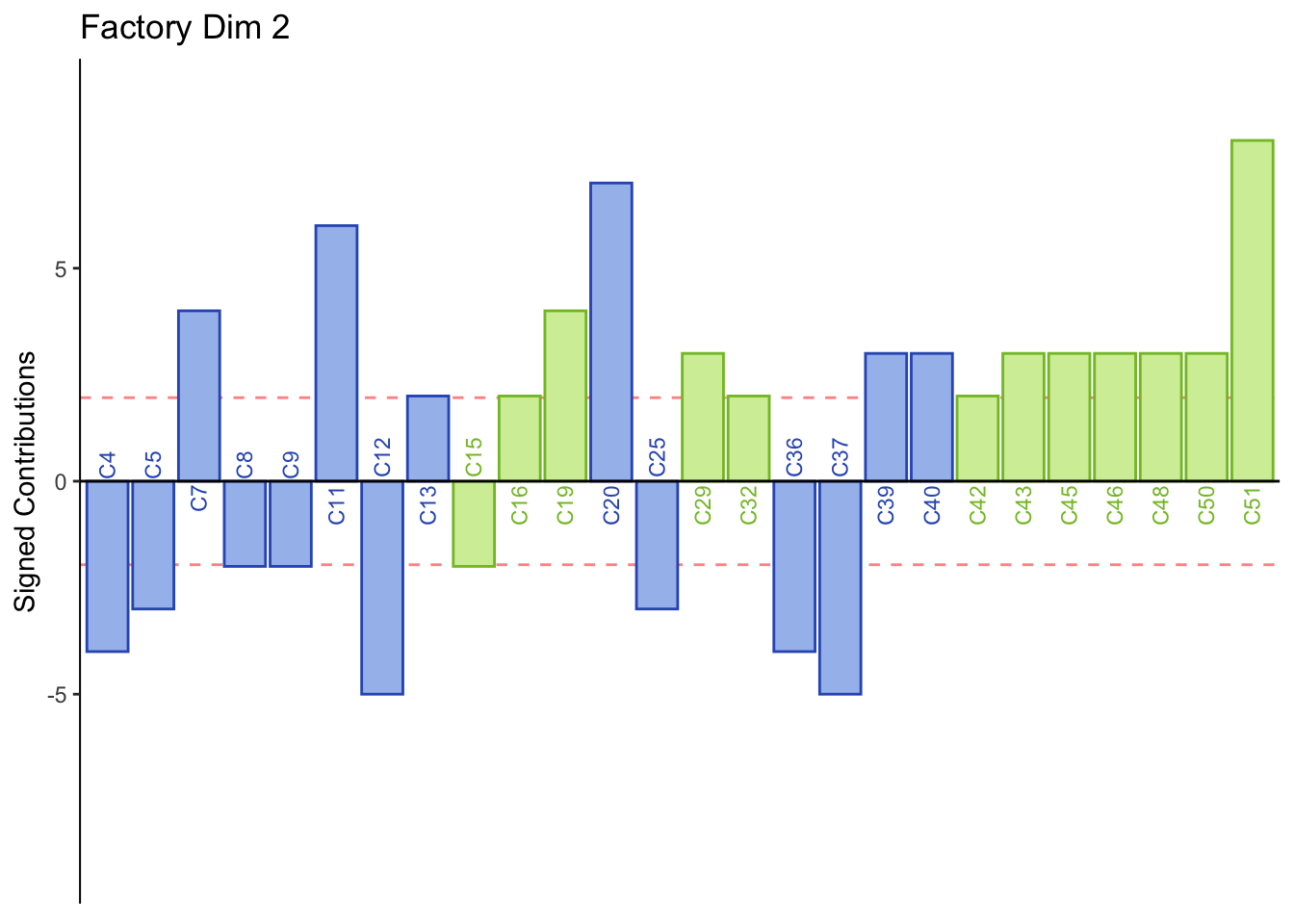
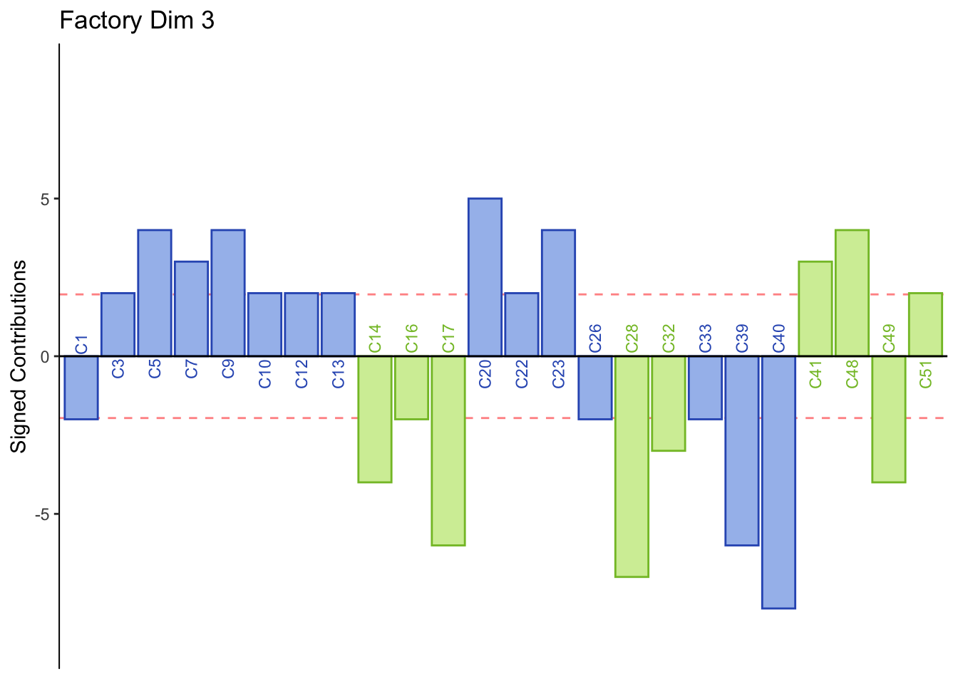
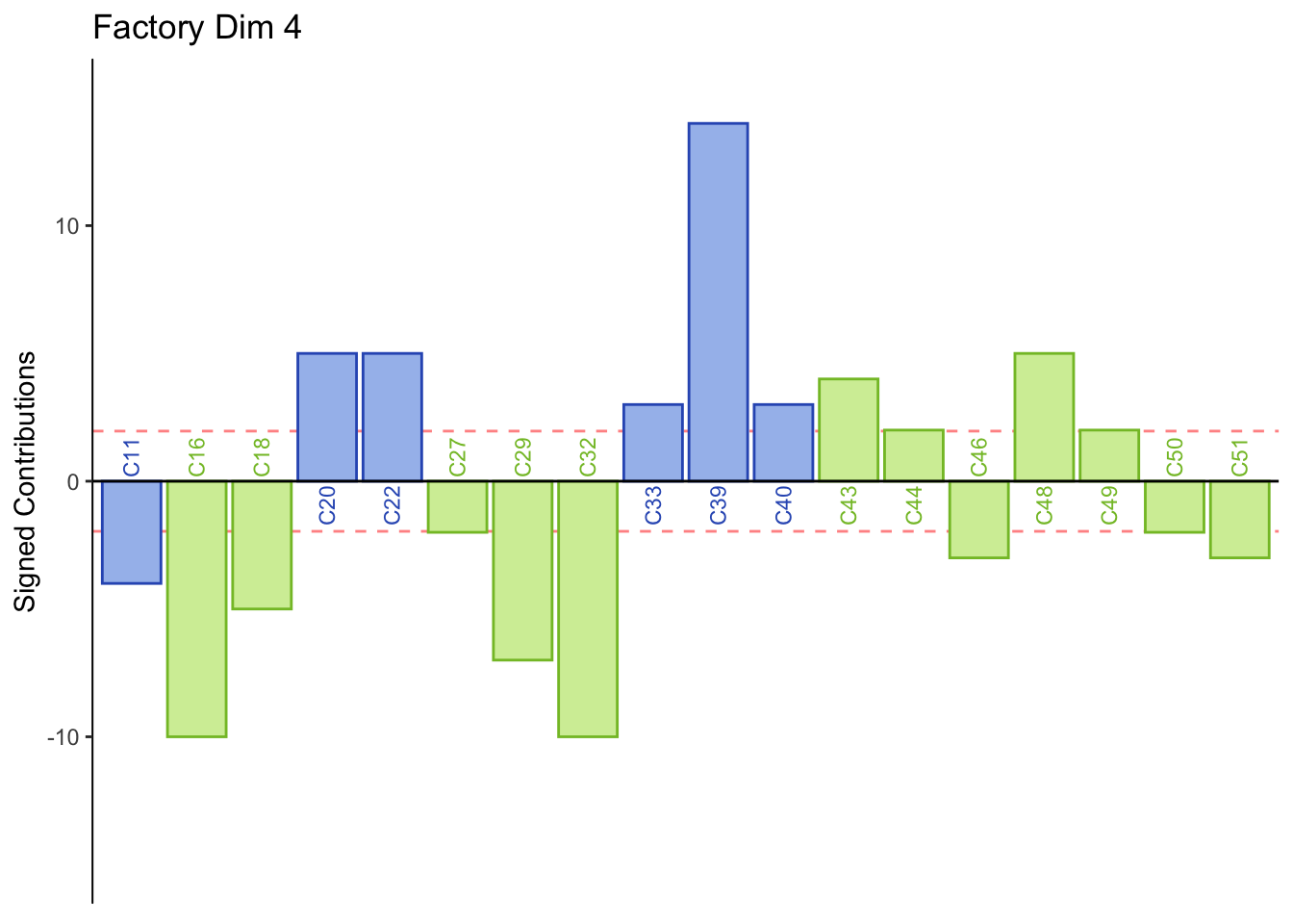
#Factory producing beer
for (k in 1:4) {
c001.plotCtrj.1F <- PrettyBarPlot2(
                       bootratio = round(100*signed.ctrj[,k]),
                       signifOnly = TRUE,
                       threshold = 100 / nrow(signed.ctrj),
                       ylim = NULL,
                       color4bar = color4IC.list$oc,
                       color4ns = "gray75",
                       plotnames = TRUE,
                       main = paste('Factory Dim', k),
                       ylab = "Signed Contributions")
print(c001.plotCtrj.1F)
#c001.plotCtrj.1 <- recordPlot()
}
8.3 Summary
Interpretations of row and column contributions together:
Dimension 1: All participants sorted mild tasting beers (group 4) together or Calavera beers (group 3) together.
Dimension 2: Females or those who consume crafted beer sorted Corona, Modelo, Tecate, and Sol together (half of group 4).
Males or those who consume industrial beer sorted Leon, Negra Modelo, Bohemia Osc adn Noche Buena together (half of group 4).
Dimension 3: Males or those who consume indudstrial beer sorted Jack, 7 Barrios, Alebrije, Ramuri, and Carolus together (group 1 and 3).
Females or those who consume crafted beer sorted Minerva and Tempus together (group 2).
Dimension 4: Females or those who consume industrial beer sorted St. Peters, Heineken, and Guiness together (group 1 and 4).
Males or those who consume crafted beer sort group 3 together.