Chapter 3 Reviewing LDA
For review of existing LDA.
Let K=5 and V = 100 possible diagnoses.
\(\theta_{i} \sim Dirichlet_5(\alpha)\)
For each of N documents per patient (let N be fixed):
- Choose a topic ID (\(z_{n} \sim multinom(\theta_i)\))
- Draw a word according to the topic-specific word distribution \((w_{n}|z_{n},\theta_i,\beta_k \sim multinom(\beta_{zn}))\)
## Loading required package: coda## Loading required package: MASS## ##
## ## Markov Chain Monte Carlo Package (MCMCpack)## ## Copyright (C) 2003-2024 Andrew D. Martin, Kevin M. Quinn, and Jong Hee Park## ##
## ## Support provided by the U.S. National Science Foundation## ## (Grants SES-0350646 and SES-0350613)
## #### simulate global distribtuion
K=5
alpha_t=5 # concentration parameter
D <- 10 # Number of pts
V = 100 # number of potential diagnoses
Theta <- rdirichlet(D,alpha = rep(alpha_t,K))
alpha_w <- 0.1 # Dirichlet parameter for topic-word distributions
beta <- rdirichlet(K,alpha = rep(alpha_w,V))
N <- 10 # Number of words in each document (assuming fixed length documents)
words <- matrix(nrow = D, ncol = N)
topic_assignments <- matrix(nrow = D, ncol = N)
## Simulate one draw from disitribtuion G_{0}
## here we use a high alpha so that the proportions are uniform with high concentration near 1/K
for(d in 1:D){
for(n in 1:N){
# Draw topic assignment z_dn
topic_assignments[d, n] <- sample(1:K, size = 1, prob = Theta[d, ])
# Draw word w_dn from the topic distribution beta_z_dn
words[d, n] <- sample(1:V, size = 1, prob = beta[topic_assignments[d,n],])
}
}But that’s not interesting! NOw the fun starts
Now we can examine the topic assignments and word distributions:
ta=melt(table(topic_assignments))
ggplot(ta,aes(topic_assignments,y=value,fill=as.factor(topic_assignments)))+geom_bar(stat="identity")+theme_classic()+labs(x="Topic Assigments",y="Frequency",fill="Topic Number")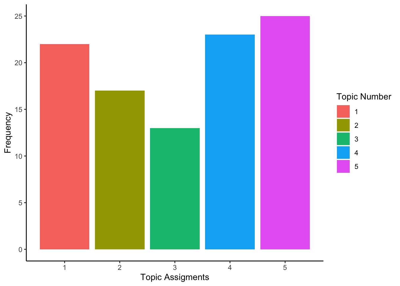
We can see the heatmap of word distribution across topics:
# Set row and column names (you may want to replace these with your actual words and topics)
row.names(beta) <- paste("Topic", 1:K)
colnames(beta) <- paste("Disease", 1:V)

# Create a custom color palette from light blue to purple
library(RColorBrewer)
my_color_palette <- brewer.pal(9, "RdPu") # Purple color palette

# Define breaks for the color scale
breaks <- seq(0, 1, length.out = 10) # Adjust as needed

# Create the heatmap without the dendrogram
heatmap(
  beta,
  col = my_color_palette,
  main = "Disease Distribution by Topic",
  xlab = "Disease",
  ylab = "Topics",
  Colv = NA,
  Rowv = NA,
  scale = "column", # Scale by column for better visualization of low and high values
  breaks = breaks,  # Define breaks for the color scale
  # Remove color scale title
  cexRow = 0.7,     # Adjust row label size
  cexCol = 0.7      # Adjust column label size
)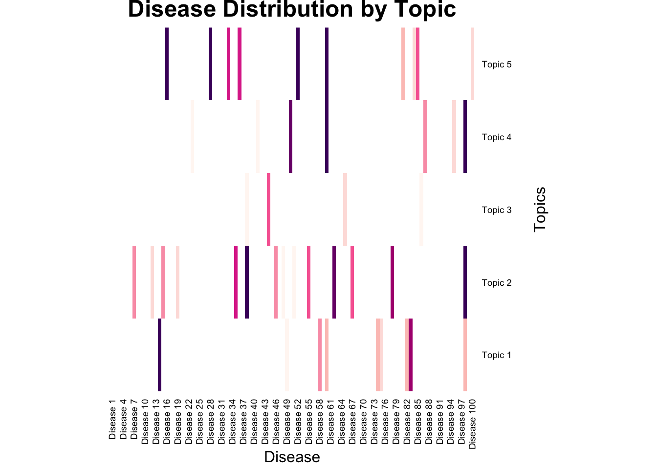
Which generates the following density of diagnoses.
Note that because we used a lower concentration parameter \(\alpha\) the distribtuion is spikier, meaning a few diseases are sampled frequently and the rest rarely.
wa=melt(table(words))
ggplot(wa,aes(words,y=value,fill=as.factor(words)))+geom_bar(stat="identity")+theme_classic()+labs(x="Disease Assignments",y="Frequency",fill="Diagnosis Number")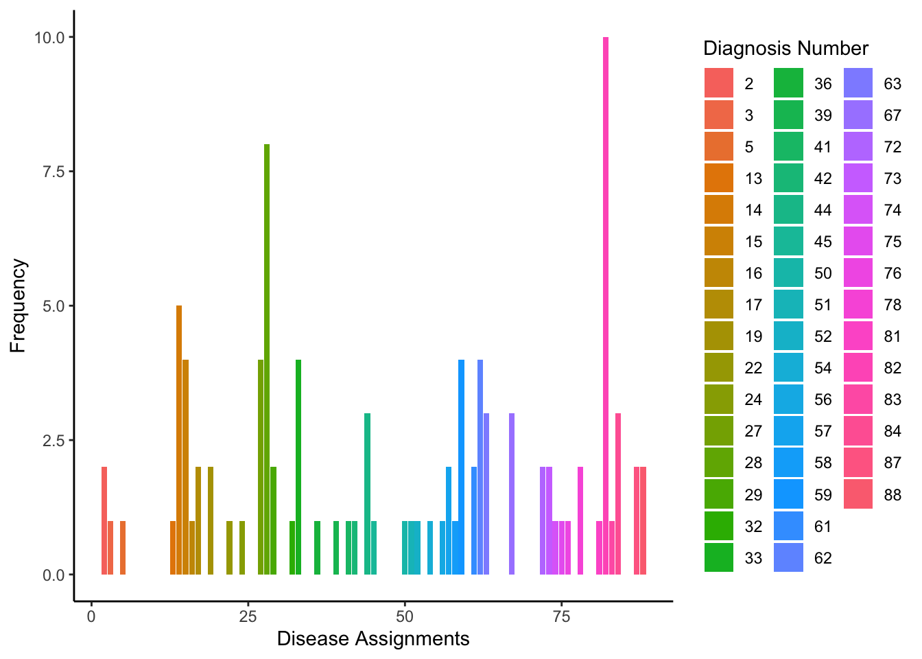
We can further summarize by topics and see that this word assignments correspond to the maximum loaded diseases within a topic:
wordlist=list()
for (i in 1:K){
  good=which(topic_assignments==i)
  wordlist[[i]]=words[good]
}


lapply(wordlist,table)
## [[1]]
##
## 2 15 16 28 32 36 56 58 75 82 88
## 2 4 1 6 1 1 1 1 1 2 2
##
## [[2]]
##
## 33 39 59 62 67 78 84 87
## 3 1 3 3 1 2 3 1
##
## [[3]]
##
## 13 27 50 63 72 73
## 1 4 1 3 2 2
##
## [[4]]
##
## 17 19 22 24 33 45 51 54 57 62 76 82 87
## 2 2 1 1 1 1 1 1 2 1 1 8 1
##
## [[5]]
##
## 3 5 14 28 29 41 42 44 52 59 61 67 74 81 83
## 1 1 5 2 2 1 1 3 1 1 2 2 1 1 1## [1] 28 90 2 88 82 14 36 32 55 16
## [1] 39 87 33 59 61 42 84 52 56 67
## [1] 27 73 4 72 18 93 10 13 63 50
## [1] 82 17 45 87 41 62 73 57 24 22
## [1] 41 28 14 67 61 29 33 44 52 80