Chapter 10 Estimating Beta
Now plot est_beta versus real:
# Assuming you have the beta array and diags list available
# Assuming you have the beta array (D x K x V x T) and individual diagnosis data (diags)

# Calculate average theta for each topic across all individuals
average_theta <- apply(Theta, 2, mean)  # Assuming Theta is D x K x T

# Calculate weighted population beta trajectories

marginal_beta=array(dim=c(D,V,T))

for (v in 1:V) {
  for (t in 1:T) {
    for (d in 1:D) {

    marginal_beta[d,v, t] <-  t(Theta[d,,t])%*%beta[d, , v, t]
  }
  }}


## weight across individuals so we have the average for everage disease and time
weighted_population_beta=apply(marginal_beta,c(2,3),mean)

# Determine individual disease onset times, create a matrix of Disease  * time
individual_onset_times =matrix(0,nrow=T,ncol=V)
  for(d in 1:D){
      for(v in 1:V){
    # Find the first time point at which the disease v is diagnosed for individual d
    onset_times <- sapply(diags[[d]], function(diag_time) v %in% diag_time)
    if (any(onset_times)) {
      individual_onset_times[which(onset_times),v]=individual_onset_times[which(onset_times),v]+1  # Return the first time point of diagnosis
    } else {
      individual_onset_times[which(onset_times),v]=individual_onset_times[which(onset_times),v]  # No diagnosis for this disease
    }}}

individual_onset_times=apply(individual_onset_times,1,function(x){x/sum(x)})


# Compare individual onset times to weighted population trajectories
# Determine individual disease onset times, create a matrix of Disease  * time
individual_onset_times_first <- sapply(1:D, function(d) {
  sapply(1:V, function(v) {
    # Find the first time point at which the disease v is diagnosed for individual d
    onset_times <- sapply(diags[[d]], function(diag_time) v %in% diag_time)
    if (any(onset_times)) {
      return(which(onset_times)[1])  # Return the first time point of diagnosis
    } else {
      return(NA)  # No diagnosis for this disease
    }
  })
})


# Function to plot population trajectories
plot_population_trajectories <- function(population_beta) {
  pop_beta_melt <- melt(t(population_beta))
  colnames(pop_beta_melt) <- c("Time", "Disease", "Probability")
  ggplot(pop_beta_melt, aes(x = Time, y = Probability, color = as.factor(Disease), group = Disease)) +
    geom_line() +
    theme_minimal() +
    labs(title = "Marginal Disease Probability Over Time for Population",
         x = "Time",
         y = "Marginal Disease Probability",
         color = "Disease")
}

library(ggplot2)
library(reshape2)


# Function to plot density of individual onset times along with population trajectories
plot_density_onset <- function(individual_onset_times, population_beta) {
  pop_beta_melt <- melt(t(population_beta))
  colnames(pop_beta_melt) <- c("Time","Disease","Probability")
  onset_melt <- melt(individual_onset_times)
  colnames(onset_melt) <- c("Disease","Time","Count")

  onset_melt <- onset_melt[!is.na(onset_melt$Count),]  # Remove NA values

  # Plot population trajectories
  p1 <- ggplot(pop_beta_melt, aes(x = Time, y = Probability, col = as.factor(Disease), group = Disease)) +
    geom_line() +
    theme_minimal() +
    labs(title = "Marginal Disease Probability Over Time for Population with Onset Time Densities",
         x = "Age",
         y = "Marginal Disease Probability",
         color = "Disease")

  # Overlay density plots for individual onset times
  p2 <- ggplot(data = onset_melt, aes(x = Time, y=Count,col = as.factor(Disease),group=Disease))+geom_smooth(fill=NA) +
    scale_color_manual(values = scales::hue_pal()(length(unique(onset_melt$Disease)))) +
    guides(color = guide_legend(override.aes = list(shape = 1)), fill = guide_legend(title = "Disease  Density"))+labs(x="Age")


    onset_melt <- melt(individual_onset_times_first)
  colnames(onset_melt) <- c("Disease", "Individual", "Time")
  onset_melt <- onset_melt[!is.na(onset_melt$Time),]  # Remove NA values

    p3 <- ggplot(data = onset_melt, aes(x = Time, fill = as.factor(Disease), alpha = 10, adjust = 1.5, position = "identity")) +geom_density()+
    scale_fill_manual(values = scales::hue_pal()(length(unique(onset_melt$Disease)))) + labs(x="Age of First Onset")+
    guides(color = guide_legend(override.aes = list(shape = 1)), fill = guide_legend(title = "Disease Onset (first) Density"))


 ggpubr::ggarrange(p1,p2,p3,common.legend = TRUE,nrow=1)
}


library(ggpubr)
plot_density_onset(individual_onset_times = individual_onset_times, population_beta = weighted_population_beta)
## `geom_smooth()` using method = 'loess' and formula = 'y ~ x'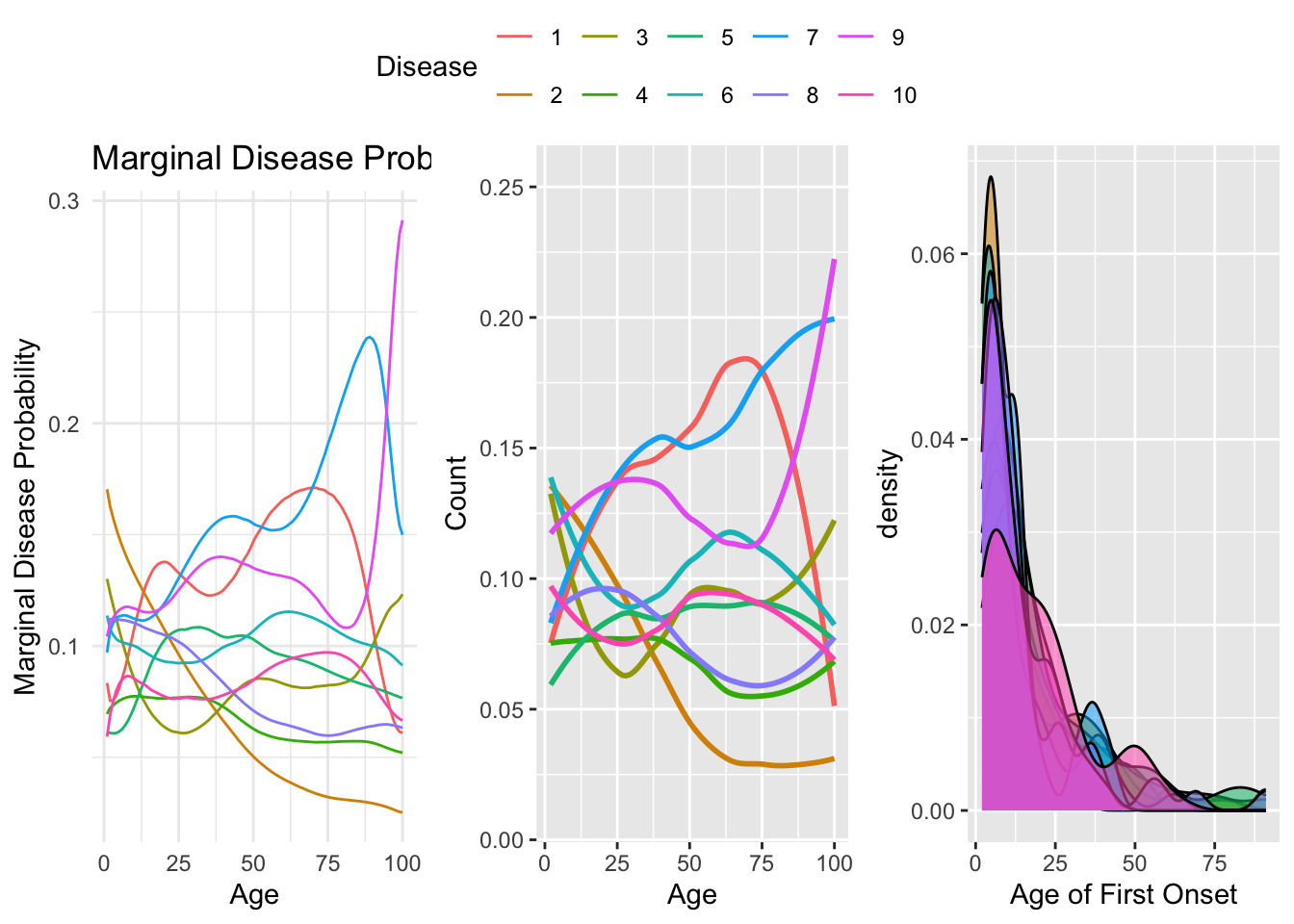
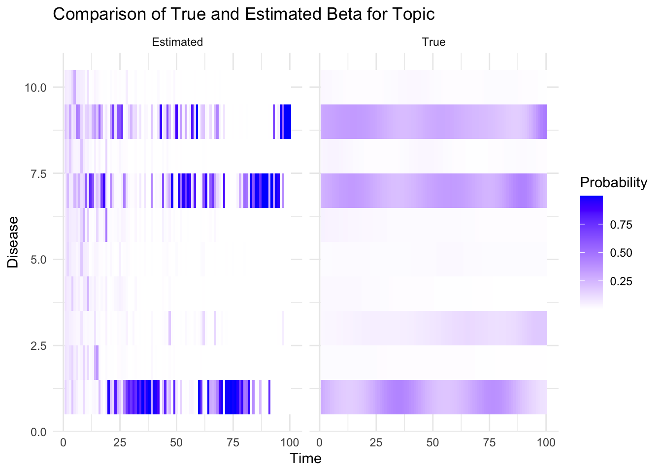
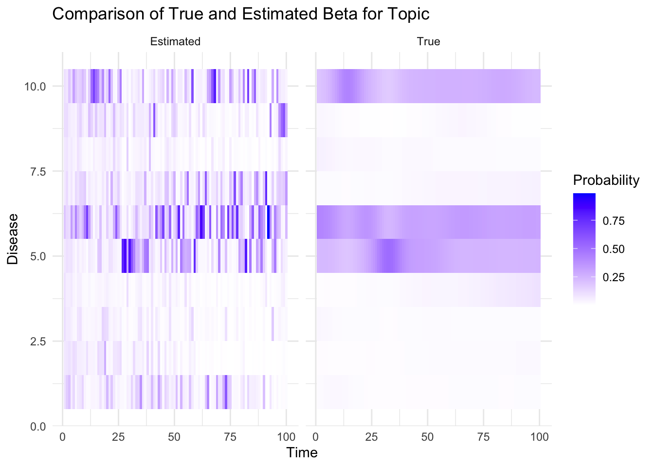
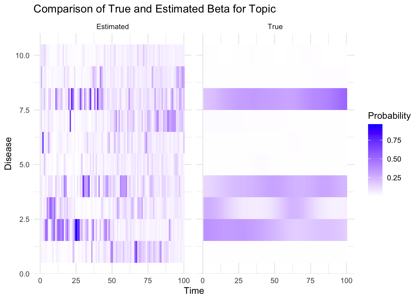
And here we try to estimate beta:
  diagnosis_counts <- array(0, dim = c(D, K, V, T))
  count_array <- array(0, dim = c(D, K, V, T))  # To keep track of the counts for averaging

  for (d in 1:D) {
    diagnoses_person <- diags[[d]]
    for (k in 1:K) {
      for (t in 1:T) {
        og_mapped_times <- which(warped_t_array[d, k, ] == t)  # Original times that map to current time t
        for (og_time in og_mapped_times) {
          diag_count <- unlist(diagnoses_person[t])
          for (w in diag_count) {
            diagnosis_counts[d, k, w, og_time] <- diagnosis_counts[d, k, w, og_time] + Theta[d, k, t]
            count_array[d, k, w, og_time] <- count_array[d, k, w, og_time] + 1
          }
        }
      }
    }
  }


## we want to make inference about popoulation beta
## plot eta with softmax and warping ....


normalize=function(x){x/sum(x)}
beta_est=apply(diagnosis_counts,c(2,3,4),sum)
for(k in 1:K){
  for(t in 1:T){
  beta_est[k,,t]=softmax_normalize(beta_est[k,,t])
  }}


true_beta=array(0,dim = c(K,V,T))
bias_value=max(eta)

  for (topic_idx in 1:K) {
    # Retrieve the diseases and their risk periods for this topic
    #specific_diseases_periods <- topic_disease_risk_periods[[topic_idx]]
    bias_increase <- disease_topic_matrix[,topic_idx]*bias_value
    for (time_idx in 1:T) {
        disease_values <- eta[topic_idx, , time_idx]

        dv <- disease_values+bias_increase

      # Apply softmax normalization
      normalized_disease <- softmax_normalize(dv)
      true_beta[topic_idx, , time_idx] <- normalized_disease
    }
  }
# Function to plot heatmaps
# Function to plot heatmaps
plot_heatmaps <- function(true_beta, est_beta,K, V, T, topic) {
true_beta_df <- melt(true_beta[topic, , ])
colnames(true_beta_df) <- c("Disease", "Time", "Probability")
true_beta_df$Type <- "True"
est_beta_df <- melt(est_beta[topic, , ])
colnames(est_beta_df) <- c("Disease", "Time", "Probability")
est_beta_df$Type <- "Estimated"
combined_df <- rbind(true_beta_df, est_beta_df)
p=ggplot(combined_df, aes(x = Time, y = Disease, fill = Probability)) +
geom_tile() +
facet_wrap(~ Type) +
scale_fill_gradient(low = "white", high = "blue") +
labs(title = "Comparison of True and Estimated Beta for Topic", topic, "and Individual",
x = "Time", y = "Disease") +
theme_minimal()
return(p)
}
# Plot heatmaps for a specific topic and individual (replace with your desired topic and individual)
plot_difference <- function(beta_est, beta_true, D, K, V, T) {
par(mfrow = c(1, 1))
# Plot difference between estimated and true beta
image(t(abs(beta_est[1, 1, , 1] - beta_true[1, 1, , 1])), main = "Difference between Estimated and True Beta", xlab = "Diseases", ylab = "Time")
}