Chapter 4 Methods: Dynamic
Remember our first objective was to model the time dependent process akin to Blei et al 2006:
In the context of dynamic topic models, we model the evolution of topic proportions or word distributions within topics over time. For a \(V\)-dimensional multinomial mean parameter \(\pi\), the \(i^{th}\) component of the natural parameter vector \(\eta_{t,k}\) for topic \(k\) at time slice \(t\) is given by \(\log(\pi_{i} / \pi_{V})\). However, unlike the Dirichlet distribution, we can employ a Gaussian Process (GP) to model this evolution in a non-parametric Bayesian framework.
A Gaussian Process defines a distribution over functions and can be used as a prior for the function space of the topic trajectories. This prior is updated with the observed data to provide a posterior distribution over the topic trajectories, allowing for smooth and flexible modeling over time. The GP is fully specified by its mean function \(\mu(t)\) and covariance function \(k(t, t')\).
In our adapted model, the evolution of each topic’s natural parameters \(\eta_{t,k}\) can be defined using a Gaussian Process:
\[ \eta_{t,k} \sim \mathcal{GP}(\mu(t), k(t, t')) \]
where \(\mu(t)\) is the mean function, and \(k(t, t')\) is the covariance function, which encodes our assumptions about the smoothness and correlation structure over time. This can capture the dynamics with more flexibility than a fixed autoregressive coefficient \(\rho\).
The mean function \(\mu(t)\) can be thought of as the ‘trend’ of the topic proportions over time, while the covariance function \(k(t, t')\) describes how these proportions change together over different time points. For example, a squared exponential covariance function will imply that the topic proportions change in a smooth manner over time.
The time-dependent natural parameters \(\eta_{t,k}\) derived from the Gaussian Process can be related back to the probability scale using the softmax function:
\[ \pi(\eta_{k,t,w}) = \frac{\exp(\eta_{k,t,w})}{\sum_{w}\exp(\eta_{k,t,w})} \]
This retains the probabilistic interpretation of topic proportions at each time step and allows for the incorporation of time-based dynamics in a principled and flexible way.
4.0.1 Time warping
Our work is complicated by the fact that \(\eta\) must not include individual level variables, so we modify the time scale and warp time:
Given a sequence of topic-word distributions over time \(\eta_{k,v,t}\) for topic \(k\), word \(v\), and time point \(t\), we introduce a time-warping function \(W(t, \rho_d)\) for individual \(d\) with a warping parameter \(\rho_d\). The warping function transforms the original time index \(t\) to a new time index \(t'\) that corresponds to the “warped” time for individual \(d\).
The warping function can be defined as:
\[ t' = W(t, \rho_d) = \left\lfloor t \cdot \rho_d \right\rfloor \]
where \(\lfloor \cdot \rfloor\) denotes the floor function which maps a real number to the largest previous integer, and \(\rho_d\) is the individual-specific warping parameter that modulates the speed at which the individual progresses through the topic content.
The “warped” topic-word distributions for individual \(d\) at time \(t'\) are then given by:
\[ \eta'_{d,k,v,t'} = \eta_{k,v,W(t, \rho_d)} \]
After applying the warping function, the resulting sequence may have gaps due to compression (when \(\rho_d < 1\)) or may need interpolation due to expansion (when \(\rho_d > 1\)). These gaps are filled using interpolation or extrapolation methods, and the resulting sequence is then normalized to ensure that it represents valid probability distributions.
The critical piece is that all individuals share the same topic-specific vocabulary, as captured in the natural parameterization of \(\eta\). Because \(\eta\) is simulated according to a dynamic topic model in which the distribtuion of a topic over diagnoses is centered at the distribtuion at the previous time step, the functions are natrually continuous.
However, we then impose a ‘warping’ to allow individuals to have disease early and late while retaining a loading on a specific topic.
4.1 Dynamic modeling: draw topics
For each of topic k, draw the natural parameters _{t,k} for the un-normlaized loadings from a MV normal with mean centrued around the natural parameters of the previous time splice.
library(MASS)
library(MCMCpack)
library(ggplot2)
#set.seed(123)

D <- 60 # number of patient

K <- 3 # Number of topics
V <- 10 # Vocabulary size
T <- 100 # Number of time slices

eta <- array(dim = c(K, V, T))

# Define a function to calculate softmax values and normalize
softmax_normalize <- function(x) {
  exp_x <- exp(x) # Subtract max to avoid overflow
  normalized_values <- exp_x / sum(exp_x)
  return(normalized_values)
}

softmax <- function(x) {
  exp_x <- exp(x) # Subtract max to avoid overflow
  normalized_values <- exp_x / sum(exp_x)
  return(normalized_values)
}
We can run in two unique ways: 1. Using a Gaussian process in which we simulate the distribtuion of proportional representation at each time step as a MV Normal with a prespecificed correlation matrix between time steps
- Using a spline as in ATM.
Here we will use the Gaussian process.
cov_function <- function(t1, t2, lengthscale, variance) {
    exp(-0.5 * (t1 - t2)^2 / lengthscale^2) * variance
}

# Store disease-specific covariances
Sigma <- array(dim = c(K, V, T, T)) # K topics, V diseases, T x T covariance matrix each


# Bias factor (adjust as needed)


# Generate covariances (adjust as needed)
for (k in 1:K) {
  for (v in 1:V) {
    # Sample a single lengthscale and variance for each topic-disease pair
      cov_matrix_kv <- matrix(0, nrow = T, ncol = T)
      #lengthscale_kv <- runif(1,min=5,max=20) ## choose random lengthscale for each topic and disease
      #variance_kv <- runif(1,0.1,0.5)## choose random variance for each topic and disease
      variance_kv=0.01 ## smaller variance means it changes less from mu funciotn

      lengthscale_kv=10
    for (i in 1:T) {
for (j in 1:T) {
        cov_matrix_kv[i, j] <- cov_function(i, j, lengthscale_kv, variance_kv)
      }
    }

    Sigma[k, v, , ] <- cov_matrix_kv
  }
}
4.2 Sample from the Gaussian Process
The probability of a disease within a topic over time has some covariance structure. We also might imagine that the disease probabilities also have some shape over time:
linear_trend <- function(time,
                         slope = 0.1,
                         intercept = 0) {
  return(slope * time + intercept)
}


logistic_growth <-
  function(t, carrying_capacity, growth_rate, t_mid) {
    carrying_capacity / (1 + exp(-growth_rate * (t - t_mid)))
  }


exponential_decay <- function(t, initial_value, decay_rate) {
  initial_value * exp(-decay_rate * t)
}

gaussian_peak <- function(t, mean, variance) {
  exp(-(t - mean) ^ 2 / (2 * variance))
}


polynomial_trend <- function(t, coefficients) {
  result <- sapply(t, function(time_point) {
    sum(sapply(1:length(coefficients), function(i) coefficients[i] * time_point^(i - 1)))
  })
  return(result)
}

sinusoidal_pattern <- function(t, amplitude, period, phase) {
  amplitude * sin((2 * pi / period) * t + phase)
}

cov_function <- function(t1, t2, lengthscale, variance) {
  return(variance * exp(-0.5 * (t1 - t2) ^ 2 / lengthscale ^ 2))
}
We might wish that each disease within a topic ihas it’s unique mean function:
# Modify eta sampling to use the correct covariance
# Covariance matrix Sigma (you should define this according to your model specifics)

time_points=1:T
# Initialize the array
topic_word_mean <- array(NA, dim = c(K, V))


mean_functions <- list(
  linear_trend = linear_trend,
  logistic_growth = logistic_growth,
  exponential_decay = exponential_decay,
  gaussian_peak = gaussian_peak,
  #polynomial_trend = polynomial_trend,
  sinusoidal_pattern = sinusoidal_pattern
)

# Define a list of names for the mean functions
mean_function_names <- names(mean_functions)


# Simulate mean functions for each disease
mu_vectors <- list()
mean_functions_called = list()


for (k in 1:K) {
  mu_vectors[[k]] <- list()
  mean_functions_called[[k]] = list()
  for (v in 1:V) {
    # Choose a mean function randomly


    # Choose a mean function by name randomly
    chosen_function_name <- sample(mean_function_names, 1)


    # Retrieve the function from the list using the name
    mean_function <- mean_functions[[chosen_function_name]]

    # Sample parameter ranges
params<- list(
  slope = runif(1, -0.05, 0.05),  # Smaller slopes for linear trend
  intercept = runif(1, -1, 1),
  carrying_capacity = runif(1, 0.5, 1.5),
  growth_rate = runif(1, 0.01, 0.1),
  t_mid = sample(time_points, 1),
  initial_value = runif(1, 0.5, 1.5),
  decay_rate = runif(1, 0.005, 0.05),
  mean = sample(time_points, 1),
  variance = runif(1, 10, 50),  # Larger variance for a flatter peak
  coefficients = runif(3, -0.1, 0.1),  # Reduce the degree and coefficient size
  amplitude = runif(1, 0.5, 1.0),
  period = sample(30:70, 1),  # More reasonable period for visible oscillations
  phase = runif(1, 0, pi)  # Limiting phase to [0, π] for simplicity
)


    # Use the appropriate parameters based on the chosen mean function
    if (chosen_function_name  == "logistic_growth") {
      function_specific_params <- list(
        t = time_points,
        carrying_capacity = params$carrying_capacity,
        growth_rate = params$growth_rate,
        t_mid = params$t_mid
      )
    } else if (chosen_function_name  == "linear_trend") {
      function_specific_params <- list(
        t = time_points,
        slope = params$slope,
        intercept = params$intercept
      )
    } else if (chosen_function_name  == "exponential_decay") {
      function_specific_params <- list(
        t = time_points,
        initial_value = params$initial_value,
        decay_rate = params$decay_rate
      )
    } else if (chosen_function_name  == "gaussian_peak") {
      function_specific_params <- list(t = time_points,
                                       mean = params$mean,
                                       variance = params$variance)
    } else if (chosen_function_name == "polynomial_trend") {
      function_specific_params <- list(t = time_points,
                                       coefficients = params$coefficients)
    } else if (chosen_function_name  == "sinusoidal_pattern") {
      function_specific_params = list(
        t = time_points,
        amplitude = params$amplitude,
        period = params$period,
        phase = params$phase
      )
    }


    # Generate the time series for the mean function using do.call
    mu_vectors[[k]][[v]] <-
      do.call(mean_function, function_specific_params)
    mean_functions_called[[k]][[v]] = list("function_name"=chosen_function_name,"params"= function_specific_params)

    eta[k, v,] <-
      mvrnorm(1, mu = mu_vectors[[k]][[v]], Sigma = Sigma[k, v, ,])
  }
}


# Normalize using softmax
eta_softmax <- array(dim = c(K, V, T))
for (k in 1:K) {
  for (t in 1:T) {
    eta_softmax[k, , t] <- softmax_normalize(eta[k, , t])
  }
}
4.3 Introduce time warping
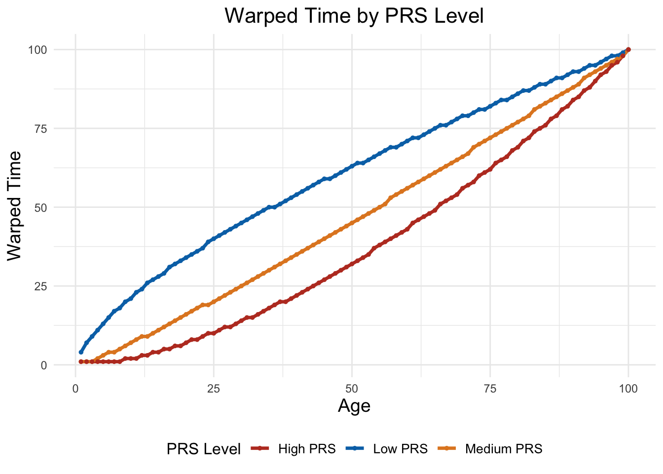
One of the unique features of our model is that individuals progress through topics at different rates according to the power of their genetic factor:
eta_tilde <- array(dim = c(D,K, V, T))

time_warping <- function(t, rho) {

  return(t^rho)
}


rho = matrix(runif(K*D,min = 0.5,max = 2),nrow=D,ncol=K)

# plot_warping_effect <- function(rho_values, t_seq = seq(0, 1, by = 0.01)) {
#  plot(t_seq, t_seq, type = 'l', lty = 2, col = 'gray', ylim = c(0, 1),
# xlab = "Original t", ylab = "Warped t", main = "Time Warping Effect")
# cols <- rainbow(length(rho_values))
# for (i in seq_along(rho_values)) {
# rho <- rho_values[i]
# lines(t_seq, time_warping(t_seq,rho), col = cols[i], lwd = 2)
# }
# legend("topright", legend = paste("rho =", rho_values), col = cols, lty = 1, cex = 0.8)
# }
#
#  plot_warping_effect(c(0.5, 1, 2))


warped_t_array <- array(0, dim = c(D, K, T))  # Initialize

for (d in 1:D) {
  for (k in 1:K) {
    for (t in 1:T) {
      warped_t <- min(T, max(1, floor(100*(time_warping(t/T, rho[d, k])))))
      warped_t_array[d, k, t] <- warped_t
    }
  }
}


for (d in 1:D) {
  for (k in 1:K) {
    for (v in 1:V) {
      for (t in 1:T) {
        warped_t <- warped_t_array[d, k, t]

        if (warped_t > T) {
          eta_tilde[d, k, v, warped_t] <- eta[k, v, T]  # Extrapolation
        } else {
          eta_values <- c()
          for (original_t in 1:T) {
            if (warped_t_array[d, k, original_t] == warped_t) {
              eta_values <- c(eta_values, eta[k, v, original_t])
            }
          }

          # Calculate average and assign so if multiple values map to warped t we will take mean
          if (length(eta_values) > 0) {
            eta_tilde[d, k, v, warped_t] <- mean(eta_values)
          } else {
            eta_tilde[d, k, v, warped_t]=NA
          }
        }
      }
    }
  }
}
for (d in 1:D) {
for (k in 1:K) {
for (v in 1:V) {
mu_pop=mu_vectors[[k]][[v]]
sigma_pop=Sigma[k, v, ,]
ind_warping_mu=mu_pop+rho[d,k]
eta_tilde[d, k, v, ]=mvrnorm(1,mu = ind_warping_mu,Sigma = sigma_pop)
}
} }The non-trivial modeling piece here is that we wish to add an individual dimension to the matrix \(\beta\) that is usually part of the topic \(\times\) disease space, and so this will make \(\beta\) an array. We are careful to keep the topic *disease** array shared across individuals, but the correlation coefficient \(\rho\) applied will be different.
4.4 From the Universal to the specific
Recall that critical to topic modeling is that eta is the same across topics. So now, we need to add the time warping feature to the individual level.
Now we need to reverse transform so that the disease proportions sum to 1.
fill_gaps <- function(values) {
  # Use na.approx from the zoo package for linear interpolation
  library(zoo)
  filled_values <- na.approx(values, na.rm = FALSE)

  # For leading NAs, use the first non-NA value
  first_non_na <- which(!is.na(filled_values))[1]
  filled_values[1:(first_non_na - 1)] <- filled_values[first_non_na]

  # For trailing NAs, use the last non-NA value
  last_non_na <- which(!is.na(filled_values))[length(which(!is.na(filled_values)))]
  filled_values[(last_non_na + 1):length(filled_values)] <- filled_values[last_non_na]

  return(filled_values[1:T])
}
# Initialize a new array for storing normalized values
beta <- array(0, dim(eta_tilde))
## since warping t isn't guaranteed to choose for every time point, we sometimes need to fill in gaps, can choose either fucntion
interpolate_spline <- function(x) {
# Identify time points with assigned values
time_with_values <- !is.na(x)
if (all(time_with_values)) {
return(x) # No interpolation needed if no NA values
} else {
# Apply spline interpolation
interpolated_values <- spline(x = which(time_with_values), y = x[time_with_values], xout = 1:length(x), method = "fmm")$y
# Replace NA values with interpolated values
x[!time_with_values] <- interpolated_values[!time_with_values]
return(x)
}
}
# Iterate through each person, topic, and time point to fill gaps and normalize
for (person_idx in 1:D) {
for (topic_idx in 1:K) {
for (v in 1:V) {
#eta_tilde[person_idx, topic_idx, v, ] <- fill_gaps(eta_tilde[person_idx, topic_idx, v, ])
eta_tilde[person_idx, topic_idx, v, ] <- interpolate_spline(eta_tilde[person_idx, topic_idx, v, ])
}}}# Target diseases for each topic
# Target diseases for each topic
topic_specific_diseases <- list()
diseases=1:V
for(k in 1:K){
sampledx=sample(diseases,size = 2,replace = F)
topic_specific_diseases[[k]]=sampledx
diseases=setdiff(diseases,sampledx)
print(length(diseases))
}## [1] 8
## [1] 6
## [1] 4# Number of topics
num_topics <- K
# Number of diseases
num_diseases <- V
bias_value=max(eta)
# Initialize the matrix with zeros
disease_topic_matrix <- matrix(0, ncol = num_topics, nrow = num_diseases)
# Loop through the list and update the matrix
for (topic_index in seq_along(topic_specific_diseases)) {
diseases <- topic_specific_diseases[[topic_index]]
# Assign 1 to the chosen diseases for the current topic
disease_topic_matrix[diseases,topic_index] <- bias_value
}
# Print the matrix
image(t(disease_topic_matrix))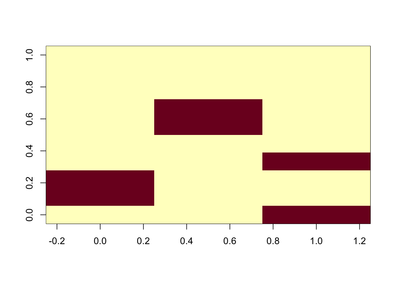
for (person_idx in 1:D) {
  for (topic_idx in 1:K) {
    # Retrieve the diseases and their risk periods for this topic
    #specific_diseases_periods <- topic_disease_risk_periods[[topic_idx]]
    active_diseases <- topic_specific_diseases[[topic_idx]]
    for (time_idx in 1:T) {
      # Assuming time_idx corresponds to actual ages, adjust as needed for your model
     # actual_age <- time_idx  # Convert time index to actual age, adjust based on your time scale

      # Find diseases that are active at this time point
      #active_diseases <- specific_diseases_periods$disease[actual_age >= specific_diseases_periods$start_age & actual_age <= specific_diseases_periods$end_age]
      #active_diseases <- topic_specific_diseases[[k]]

      disease_values <- eta_tilde[person_idx, topic_idx, , time_idx]

      # Increase the values for active diseases at this time before normalization
      if (length(active_diseases) > 0) {
        disease_values[active_diseases] <- disease_values[active_diseases] + bias_value
      }

      # Apply softmax normalization
      normalized_disease <- softmax_normalize(disease_values)
      beta[person_idx, topic_idx, , time_idx] <- normalized_disease
    }
  }
}


which(order(apply(beta[,1,,],2,mean),decreasing = T)%in%(topic_specific_diseases[[1]])==TRUE)
## [1] 1 2## [1] 1 2## [1] 1 2# 'beta' now contains the softmax-normalized disease values, and they should sum to 1 for each person, topic, and time point.beta <- array(0, dim(eta_tilde))
# Determine the number of topics in which each disease will be primarily active
#num_topics_per_disease <- sample(1:2, V, replace = TRUE) # Each disease is active in 1 or 2 topics
num_topics_per_disease = rep(1,V)
# Initialize the list to store the primary topics for each disease
disease_primary_topics <- vector("list", length = V)
# Initialize the disease-topic matrix with zeros indicating inactivity
disease_topic_matrix <- matrix(0, nrow = V, ncol = K)
# Assign primary topics to each disease
for (disease in 1:V) {
primary_topics <- sample(1:K, num_topics_per_disease[disease])
disease_primary_topics[[disease]] <- primary_topics
# Set the bias value for the disease in its primary topics, can vary
#bias_values <- runif(num_topics_per_disease[disease], 0, 1) # Variable bias between 0 and 1
bias_values = rep(1,num_topics_per_disease[disease])
# Fill in the disease-topic matrix with bias values for the primary topics
disease_topic_matrix[disease, primary_topics] <- bias_values
}
image(t(disease_topic_matrix))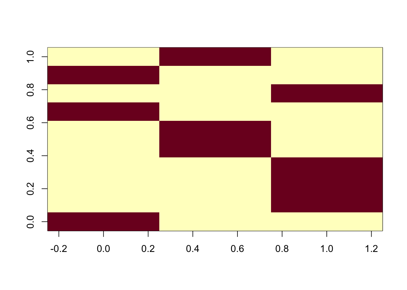
bias_value=max(eta)

for (person_idx in 1:D) {
  for (topic_idx in 1:K) {
    # Retrieve the diseases and their risk periods for this topic
    #specific_diseases_periods <- topic_disease_risk_periods[[topic_idx]]
    bias_increase <- disease_topic_matrix[,topic_idx]*bias_value
    for (time_idx in 1:T) {
      # Assuming time_idx corresponds to actual ages, adjust as needed for your model
     # actual_age <- time_idx  # Convert time index to actual age, adjust based on your time scale

      # Find diseases that are active at this time point
      #active_diseases <- specific_diseases_periods$disease[actual_age >= specific_diseases_periods$start_age & actual_age <= specific_diseases_periods$end_age]
      #active_diseases <- topic_specific_diseases[[k]]

      disease_values <- eta_tilde[person_idx, topic_idx, , time_idx]

      # Increase the values for active diseases at this time before normalization
        dv <- disease_values+bias_increase

      # Apply softmax normalization
      normalized_disease <- softmax_normalize(dv)
      beta[person_idx, topic_idx, , time_idx] <- normalized_disease
    }
  }
}library(ggplot2)
library(reshape2)
# Example data (replace with your actual data)
# Selecting the indices for different PRS levels
low_prs_index <- which(rho[,k] < 0.7)[1]
medium_prs_index <- which(rho[,k] > 0.8 & rho[,k] < 1.2)[1]
high_prs_index <- which(rho[,k] > 1.3)[1]
# Creating a data frame from the warped time array
warped_t_data <- data.frame(
Age = rep(1:100, 3),
Warped_Time = c(warped_t_array[low_prs_index, k, ],
warped_t_array[medium_prs_index, k, ],
warped_t_array[high_prs_index, k, ]),
PRS_Level = factor(rep(c("Low PRS", "Medium PRS", "High PRS"), each = 100))
)
# Plotting using ggplot2
ggplot(warped_t_data, aes(x = Age, y = Warped_Time, color = PRS_Level)) +
geom_line(size = 1.2) +
geom_point(size = 1) +
labs(
title = "Warped Time by PRS Level",
x = "Age",
y = "Warped Time",
color = "PRS Level"
) +
theme_minimal() +
scale_color_nejm() +
theme(
plot.title = element_text(hjust = 0.5, size = 16),
axis.title = element_text(size = 14),
legend.position = "bottom",
legend.title = element_text(size = 12),
legend.text = element_text(size = 10)
)