Chapter 5 Using EMC2 for EAMs I - DDM
5.1 DDM
In this chapter, we include a detailed overview for fitting the DDM using EMC2. The DDM is the most commonly used EAM, with the model being used to account for a wide variety of decision making behaviours, such as recognition memory, working memory, speed-accuracy trade-off, word recognition and cognitive control. A graphical example of the DDM as a decision model can be seen below.
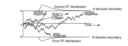
Figure 5.1: The diffusion decision model
5.1.1 Parameterisation and Transformations
The “TZD” parameterisation of the DDM, which is defined relative to the “rtdists” package as having parameters on the natural scale, log scale and the probit scale. On the natural scale are drift rates (v) where positive values favors upper boundaries. On the log scale, all parameters are assumed to be greater than 0. These include; non-decision time (t0) as the lower bound of non-decision time, width of non-decision time distribution (st0), upper threshold (a), standard deviation of v (sv), and moment-to-moment standard deviation (s). On the probit scale, all values fall between 0 and 1. For this, we have start point z which is given by Z*a (i.e., estimate Z), start-point variability which is given by sz = 2*SZ*min(c(a*Z,a*(1-Z)) (i.e., estimate SZ) and d given by d = t0(upper)-t0(lower) = (2*DP-1)*t0 (i.e., estimate DP).
Lets now look at an example of using the DDM.
5.2 Setup
Let’s first explore the data. For this example, we’re using the same data as the previous example from Forstmann et al. (2008). When we explore the data, we can check the number of subjects, trials per subject and factors across the data.
rm(list=ls())
source("emc/emc.R")
source("models/DDM/DDM/ddmTZD.R")


#### Format the data to be analyzed ----

print(load("Data/PNAS.RData"))
# Note that this data was censored at 0.25s and 1.5s

dat <- data[,c("s","E","S","R","RT")]
names(dat)[c(1,5)] <- c("subjects","rt")
levels(dat$R) <- levels(dat$S)

#### Explore the data ----

# 3 x 2 design, 19 subjects
lapply(dat,levels)

# 800 trials per subject
table(dat$subjects)

# 70-90% accuracy, .35s - .5s mean RT
plot_defective_density(dat,factors=c("E","S"),layout=c(2,3))
## $subjects
## [1] "as1t" "bd6t" "bl1t" "hsft" "hsgt" "kd6t" "kd9t" "kh6t" "kmat" "ku4t" "na1t"
## [12] "rmbt" "rt2t" "rt3t" "rt5t" "scat" "ta5t" "vf1t" "zk1t"
##
## $E
## [1] "accuracy" "neutral" "speed"
##
## $S
## [1] "left" "right"
##
## $R
## [1] "left" "right"
##
## $rt
## NULL##
## as1t bd6t bl1t hsft hsgt kd6t kd9t kh6t kmat ku4t na1t rmbt rt2t rt3t rt5t scat ta5t
## 810 849 843 848 849 849 849 837 846 845 848 831 842 843 691 849 845
## vf1t zk1t
## 838 806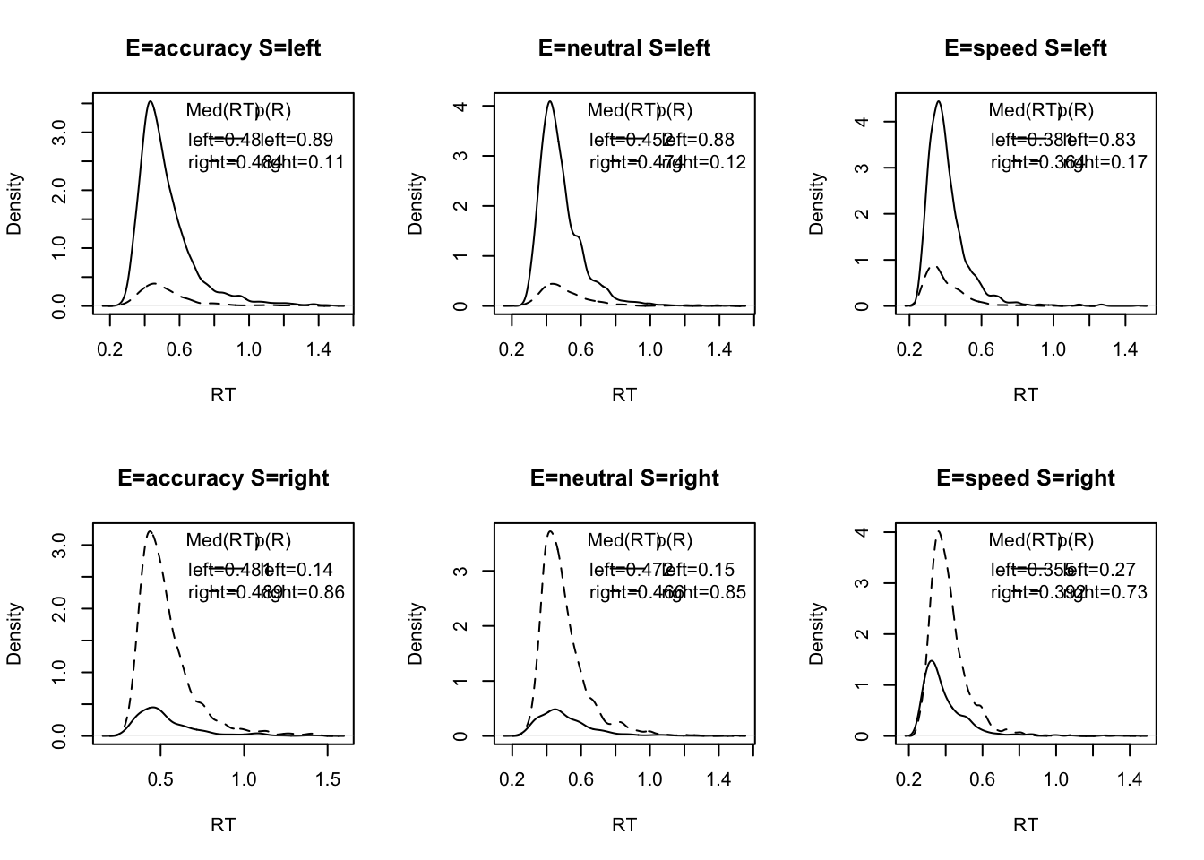
Here we’ve plotted the “defective density” across emphasis and stimuli conditions. By doing this, we can see the distribution of response times for both correct and error responses. In this example, using EAMs, we aim to estimate bivariate data - that is, both response time and responses, so it is important to evaluate this data conjointly when first looking at the data.
5.3 Set up the design
Now we can start thinking about some simple effects for the DDM. In this example, we’re going to show some more detailed contrasts for effects in the data. In this experiment, the main effect of interest was for the emphasis manipulation, where participants were instructed to respond more accurately or more quickly (or by balancing both of these components).
For the emphasis factor, there are three conditions; speed, accuracy and neutral. In this example, we are interested in the differences between these conditions. For the contrast matrix, condition 1 is accuracy, so there is no contrast for this cell. Condition 2 in neutral, so we do accuracy - neutral (for the parameter difference), and condition 3 is speed, so again we need the difference parameter.
For the matching/mismatching drift rates, we need a test stimulus factor with an intercept term and right-left factor. When applied to rate parameter v_S is the traditional DDM “drift rate” parameter. The intercept term is drift bias. If it is zero, drift rate is the same for left and right. If positive, the rate bias favors right, when negative, it favors left. For example, intercept v = 1, v_S = 2 implies an upper rate of 3 and lower rate of -1.
#### Set up the design ----

Emat <- matrix(c(0,-1,0,0,0,-1),nrow=3)
dimnames(Emat) <- list(NULL,c("a-n","a-s"))


Vmat <- matrix(c(-1,1),ncol=1,dimnames=list(NULL,""))
Here we set up two contrasts - one for emphasis and one for drift rate. Let’s look at how these look, starting with the emphasis matrix;
##      a-n a-s
## [1,]   0   0
## [2,]  -1   0
## [3,]   0  -1
And the drift bias matrix;
##
## [1,] -1
## [2,]  1
Now we can use these to set up our model.
5.4 Wiener diffusion model
In this example, we use a Wiener diffusion model where the between-trial variability parameters are set to zero in “constants” (Note: this is done on the “sampled” scale, so we do a probit transform for DP and SZ and log for st0 and sv). We also include the traditional characterization of the speed vs. accuracy emphasis factor (E) selectively influencing threshold (a), and stimulus (S) affecting rate (v). In order to make the model identifiable we set moment-to-moment variability to the conventional value of 1.
Using our EMC2 arguments as we have done previously, we include factors of subject, stimulus (S) and emphasis (E) in our factors list. We also include the response levels and contrasts that we created earlier. For this example, we have effects of S (stimuli) on v (drift) and effect of E (emphasis conditions) on a (threshold/boundary separation), with no effects on the other parameters. For the constants, we include constants for s, st0, DP, SZ and sv – for these we refer to the scale identified above. When we do this, we can now check our parameters to be sampled.
design_a <- make_design(
  Ffactors=list(subjects=levels(dat$subjects),S=levels(dat$S),E=levels(dat$E)),
  Rlevels=levels(dat$R),
  Clist=list(S=Vmat,E=Emat),
  Flist=list(v~S,a~E,sv~1, t0~1, st0~1, s~1, Z~1, SZ~1, DP~1),
  constants=c(s=log(1),st0=log(0),DP=qnorm(0.5),SZ=qnorm(0),sv=log(0)),
  model=ddmTZD)
## v v_S a a_Ea-n a_Ea-s t0 Z
## 0 0 0 0 0 0 0
## attr(,"map")
## attr(,"map")$v
## v v_S
## 1 1 -1
## 20 1 1
##
## attr(,"map")$a
## a a_Ea-n a_Ea-s
## 1 1 0 0
## 39 1 -1 0
## 77 1 0 -1
##
## attr(,"map")$sv
## sv
## 1 1
##
## attr(,"map")$t0
## t0
## 1 1
##
## attr(,"map")$st0
## st0
## 1 1
##
## attr(,"map")$s
## s
## 1 1
##
## attr(,"map")$Z
## Z
## 1 1
##
## attr(,"map")$SZ
## SZ
## 1 1
##
## attr(,"map")$DP
## DP
## 1 1# This produces a 7 parameter model
sampled_p_vector(design_a)## v v_S a a_Ea-n a_Ea-s t0 Z
## 0 0 0 0 0 0 0
## attr(,"map")
## attr(,"map")$v
## v v_S
## 1 1 -1
## 20 1 1
##
## attr(,"map")$a
## a a_Ea-n a_Ea-s
## 1 1 0 0
## 39 1 -1 0
## 77 1 0 -1
##
## attr(,"map")$sv
## sv
## 1 1
##
## attr(,"map")$t0
## t0
## 1 1
##
## attr(,"map")$st0
## st0
## 1 1
##
## attr(,"map")$s
## s
## 1 1
##
## attr(,"map")$Z
## Z
## 1 1
##
## attr(,"map")$SZ
## SZ
## 1 1
##
## attr(,"map")$DP
## DP
## 1 1From this output, we can see the parameter vector to estimate, as well as the contrasts used for each individual parameter. For the to-be-sampled parameters, v is the rate intercept, and v_S the traditional drift rate, a is the threshold for accuracy, a_Ea-n accuracy-neutral and a_Ea-s accuracy - neutral. t0 is the mean non-decision time and Z the proportional start-point bias (note that unbiased Z = 0.5).
5.5 Hierarchical Fitting
For this example, we fit a “standard” hierarchical model that allows for population correlations among all parameters (7 x (7-1) /2 = 21 correlations), along with population mean (mu) and variance estimates for each parameter. Note that in the previous chapter, we mainly focused on fitting single subjects or using “independent” group level models, where no relations were assumed between parameters. However, this assumption is rarely accurate in hierarchical model-based sampling, especially for cognitive models. Hence, the standard EMC2 fitting method provides an advance on other hierarchical samplers as we are able to easily estimate a group level model that accounts for parameter correlations. In the following chapter, we’ll take more time to discuss hierarchical modelling and PMwG sampling, however, for now, let’s just focus on the EAM.
5.5.1 Prior setting
Here we use the default hyper-prior, reproduced here explicitly (the same is obtained if the prior argument is omitted from make_samplers). It sets a mean of zero and a variance of 1 for all parameters and assumes they are independent.
In EMC2, we make setting priors straightforward, and there is less requirement from the user to think about priors on each parameter (compared to DMC or STAN). Many of the models have built-in priors, and hyper-priors are generally non-informative. We plan to add informed priors into EMC2 in the future. In the following chapter, we will also discuss priors for EMC2 and PMwG.
prior=list(theta_mu_mean = rep(0, 7), theta_mu_var = diag(rep(5, 7)))
prior
## $theta_mu_mean
## [1] 0 0 0 0 0 0 0
##
## $theta_mu_var
## [,1] [,2] [,3] [,4] [,5] [,6] [,7]
## [1,] 5 0 0 0 0 0 0
## [2,] 0 5 0 0 0 0 0
## [3,] 0 0 5 0 0 0 0
## [4,] 0 0 0 5 0 0 0
## [5,] 0 0 0 0 5 0 0
## [6,] 0 0 0 0 0 5 0
## [7,] 0 0 0 0 0 0 55.6 Prepare the sampler
Now we can take the data, our design and our priors and look to estimate the model. The make_samplers function combines the data and design and makes a list of n_chains pmwg objects ready for sampling. Here we use the default 3 chains. Each will be sampled independently (multiple chains are useful for assessing convergence). We’ll go over the use of chains in the next chapter, but for now lets get to sampling!
samplers <- make_samplers(dat,design_a,type="standard",
                          prior_list=prior,n_chains=3,rt_resolution=.02)
save(samplers,file="sPNAS_a.RData")
5.7 Estimate the model
Note Running this code will take a significant amount of computer power (6 cpus) and may take several minutes-hours depending on the computer. We recommend sourcing the supplied examples if you are following along with the code. This can be done by saving the samples from OSF to your desktop and using; load("Desktop/osfstorage-archive/DDM/sPNAS_a.RData")
The following code samples for all three stages of the sampling scheme (explained in detail in the following chapter), before using the post_predict function to generate posterior predicted data from the estimated model. Notice at each step we save the sampled object - this is so that we can avoid having to re-run parts of the code if there is a bug at any stage (as this will generally be run on a computer grid).
source("emc/emc.R")
source("models/DDM/DDM/ddmTZD.R")


sPNAS_a <- run_burn(samplers,cores_per_chain=2)
save(sPNAS_a,file="sPNAS_a.RData")
sPNAS_a <- run_adapt(sPNAS_a,cores_per_chain=2)
save(sPNAS_a,file="sPNAS_a.RData")
sPNAS_a <- run_sample(sPNAS_a,iter=1000,cores_per_chain=2)
save(sPNAS_a,file="sPNAS_a.RData")
ppPNAS_a <- post_predict(sPNAS_a,n_cores=19)
save(ppPNAS_a,sPNAS_a,file="sPNAS_a.RData")
Lets explore the fitting script a little further. Fitting is performed in the script Desktop/osfstorage-archive/DDM/sPNAS_a.R (e.g., on a linux based system the command line is R CMD BATCH sPNAS_a.R & to run it in background). We use three procedures that run the “burn”, “adapt” and “sample” until they produce samples with the required characteristics. By default each chain gets its own cores (this can be set with the cores_for_chains argument) and the cores_per_chain argument above gives each chain 2 cores, so 6 are used in total. Below are the functions called by sPNAS_a.R.
The first “burn” stage (sPNAS_a <- run_burn(samplers,cores_per_chain=2)) by default runs 500 iterations, discards the first 200 and repeatedly trys adding new iterations (and possibly removing initial) iterations until R hat is less than a criterion (1.1 by default) for all random effect parameters in all chains. The aim of this stage is to find the posterior mode and get chains suitable for the next “adapt” stage.
The “adapt” stage (sPNAS_a <- run_adapt(sPNAS_a,cores_per_chain=2)) develops and approximation to the posterior that will make sampling more efficient (less autocorrelated) in the final “sample” stage.
Here in the final sample stage (sPNAS_a <- run_sample(sPNAS_a,iter=1000,cores_per_chain=2)) we ask for 1000 iterations per chain.
Once sampling is completed the script also gets posterior predictive samples(ppPNAS_a <- post_predict(sPNAS_a,n_cores=19)) to enable model fit checks. By default this is based on randomly selecting iterations from the final (sample) stage, and provides posterior predictives for the random effects. Here we use one core pre participant.
5.8 Results and checks
Lets load in the results and look at them.
load("~/Desktop/emc2/models/DDM/DDM/examples/samples/sPNAS_a.RData")5.8.1 Check convergence
We can first check the state of samplers;
chain_n(sPNAS_a)## burn adapt sample
## [1,] 500 120 1000
## [2,] 500 120 1000
## [3,] 500 120 1000We can see that each chain ran the same amount of iterations for all three stages - this is because by default, EMC2 will trim each object or increase the number of iterations such that the samples are of matching length.
Lets now look at the chains for the burn samples. For chain plots, we first look at the likelihood values for each subject. These values should increase at the start of sampling and then find some stationarity across chains. If the chains don’t converge, then there is likely a problem with the model - such as a local maxima being found.
plot_chains(sPNAS_a,selection="LL",layout=c(4,5),filter="burn")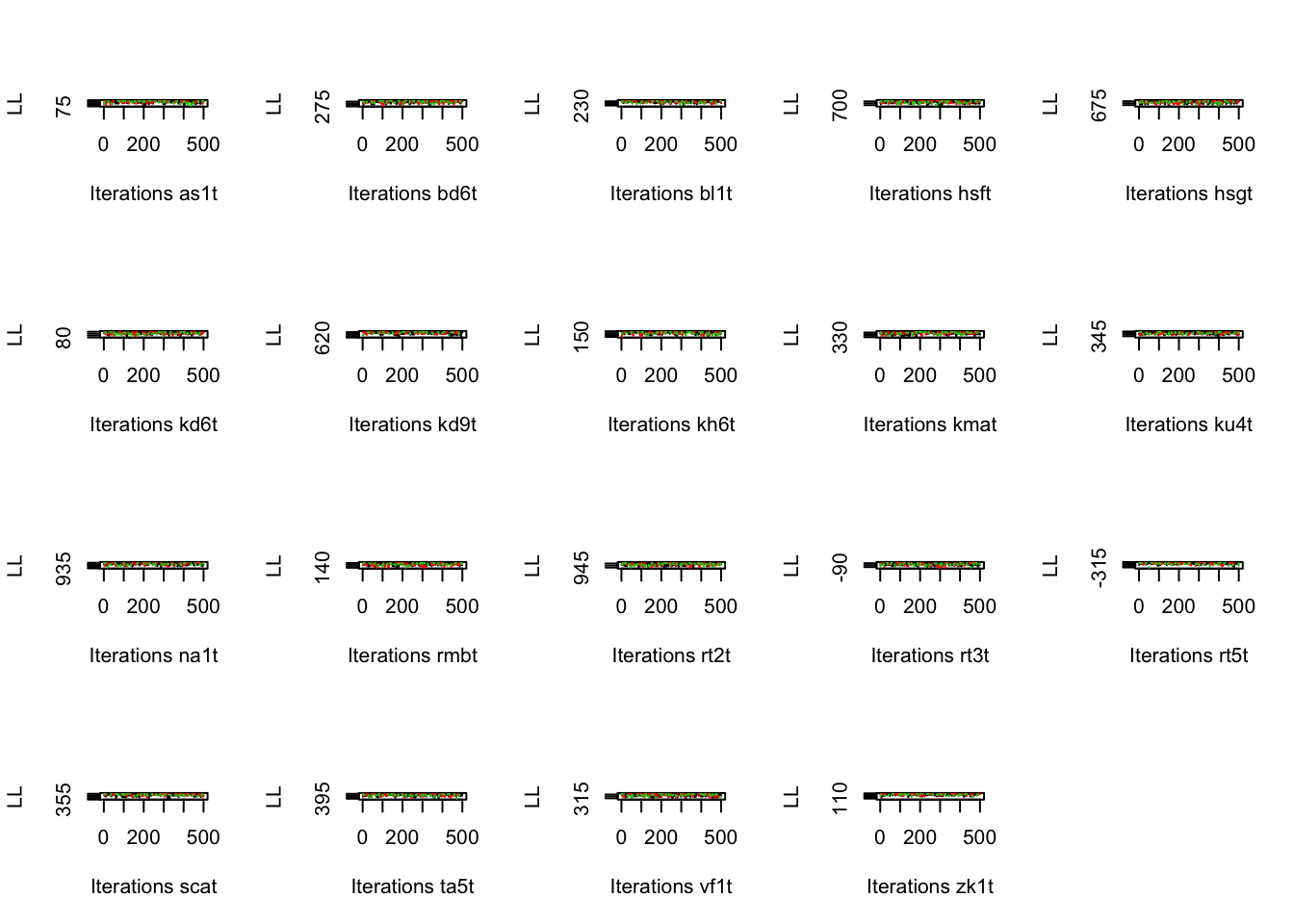
Next, we can look at the parameter chains for each subject (we won’t do that here though as it will take up a lot of space and we’d rather save the trees).
par(mfrow=c(2,7))
plot_chains(sPNAS_a,selection="alpha",layout=NULL,filter="burn")
As another check of convergence, lets look at the Gelman diag statistic across subjects. Notice here that we filter burn-in.
# R hat indicates mostly good mixing
gd_pmwg(sPNAS_a,selection="alpha",filter="burn")
## bl1t kd9t rt3t kmat kh6t rmbt as1t bd6t scat zk1t hsgt kd6t ta5t vf1t na1t rt5t hsft
## 1.01 1.02 1.02 1.02 1.02 1.02 1.02 1.03 1.03 1.03 1.04 1.04 1.05 1.05 1.05 1.06 1.06
## rt2t ku4t
## 1.07 1.08Now lets check convergence across subjects and parameters;
# Default shows multivariate version over parameters. An invisible return
# provides full detail, here printed and rounded, again very good
round(gd_pmwg(sPNAS_a,selection="alpha",filter="burn",print_summary = FALSE),2)
## v v_S a a_Ea-n a_Ea-s t0 Z mpsrf
## as1t 1.01 1.00 1.01 1.02 1.00 1.01 1.00 1.02
## bd6t 1.00 1.00 1.00 1.01 1.01 1.00 1.02 1.03
## bl1t 1.00 1.00 1.00 1.01 1.00 1.01 1.02 1.01
## hsft 1.02 1.00 1.01 1.02 1.00 1.01 1.06 1.06
## hsgt 1.03 1.00 1.00 1.01 1.00 1.00 1.03 1.04
## kd6t 1.02 1.01 1.02 1.03 1.02 1.00 1.03 1.04
## kd9t 1.01 1.00 1.00 1.01 1.01 1.02 1.01 1.02
## kh6t 1.00 1.00 1.00 1.02 1.01 1.01 1.00 1.02
## kmat 1.01 1.01 1.00 1.00 1.01 1.01 1.02 1.02
## ku4t 1.08 1.00 1.00 1.00 1.00 1.00 1.08 1.08
## na1t 1.01 1.01 1.02 1.05 1.03 1.01 1.01 1.05
## rmbt 1.00 1.00 1.00 1.04 1.00 1.00 1.01 1.02
## rt2t 1.01 1.00 1.02 1.04 1.01 1.00 1.04 1.07
## rt3t 1.01 1.00 1.01 1.00 1.01 1.02 1.01 1.02
## rt5t 1.00 1.00 1.01 1.05 1.00 1.01 1.01 1.06
## scat 1.02 1.00 1.01 1.01 1.00 1.02 1.04 1.03
## ta5t 1.02 1.00 1.01 1.03 1.01 1.00 1.02 1.05
## vf1t 1.01 1.00 1.01 1.06 1.01 1.02 1.02 1.05
## zk1t 1.01 1.00 1.02 1.04 1.01 1.01 1.02 1.03So we can feel pretty secure that the estimation did a good job of reaching the posterior mode - great! Now we can focus on the sample stage, where the samples we use for inference will come from. These samples are drawn from the posterior in an efficient way. The default setting for the filter argument across EMC2 functions is set to sample stage.
Let’s first look at the random effects - i.e., the subject level parameters (alpha) - for the sampled (final) stage.
# Participant likelihoods all fat flat hairy caterpillars
plot_chains(sPNAS_a,selection="LL",layout=c(4,5))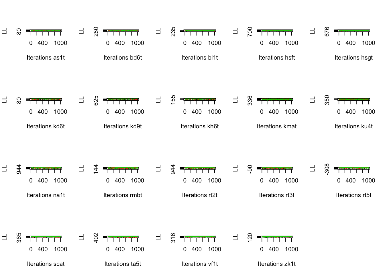
Again we’re not going to take up too much space, but you should plot the parameter chains per subject as below;
# Plot random effects (default selection="alpha"), again they look good
par(mfrow=c(2,7)) # one row per participant
plot_chains(sPNAS_a,selection="alpha",layout=NULL)
Next we’re going to look at the chain mixing using the same Gelman diag statistic as above.
# MIXING
# R hat indicates excellent mixing
round(gd_pmwg(sPNAS_a,selection="alpha",print_summary = FALSE),2)
## v v_S a a_Ea-n a_Ea-s t0 Z mpsrf
## as1t 1 1 1 1 1 1.00 1 1.00
## bd6t 1 1 1 1 1 1.00 1 1.01
## bl1t 1 1 1 1 1 1.00 1 1.00
## hsft 1 1 1 1 1 1.00 1 1.00
## hsgt 1 1 1 1 1 1.00 1 1.00
## kd6t 1 1 1 1 1 1.00 1 1.00
## kd9t 1 1 1 1 1 1.00 1 1.01
## kh6t 1 1 1 1 1 1.00 1 1.00
## kmat 1 1 1 1 1 1.00 1 1.00
## ku4t 1 1 1 1 1 1.00 1 1.00
## na1t 1 1 1 1 1 1.00 1 1.00
## rmbt 1 1 1 1 1 1.00 1 1.00
## rt2t 1 1 1 1 1 1.00 1 1.00
## rt3t 1 1 1 1 1 1.00 1 1.01
## rt5t 1 1 1 1 1 1.00 1 1.00
## scat 1 1 1 1 1 1.03 1 1.00
## ta5t 1 1 1 1 1 1.00 1 1.00
## vf1t 1 1 1 1 1 1.00 1 1.00
## zk1t 1 1 1 1 1 1.00 1 1.00We can also look at the sampling efficiency. The effective number of samples can give you an idea of the autocorrelation present within the sampling, where we try to avoid high autocorrelation (which generally indicates a problem with the model).
# Actual number samples = 3 chains x 533 per chain = 1599.
# The average effective number shows autocorrelation is quite low
round(es_pmwg(sPNAS_a,selection="alpha"))
## a_Ea-n Z v a a_Ea-s t0 v_S
## 1619 1818 2026 2334 2437 2631 2649## v v_S a a_Ea-n a_Ea-s t0 Z
## 2026 2649 2334 1619 2437 2631 1818Sometimes you might want to look at worst case summary;
round(es_pmwg(sPNAS_a,selection="alpha",summary_alpha=min))## a_Ea-n Z v a t0 a_Ea-s v_S
## 820 1166 1431 1737 1816 1843 2153## v v_S a a_Ea-n a_Ea-s t0 Z
## 1431 2153 1737 820 1843 1816 1166Or get per subject details;
round(es_pmwg(sPNAS_a,selection="alpha",summary_alpha=NULL))## [1] 820 1075 1166 1175 1290 1323 1399 1423 1431 1436 1458 1474 1475 1498 1510 1526
## [17] 1535 1547 1577 1600 1702 1724 1725 1728 1737 1739 1749 1763 1776 1796 1797 1816
## [33] 1841 1843 1862 1872 1902 1907 1945 1976 1982 1984 1992 2016 2027 2041 2045 2059
## [49] 2078 2103 2109 2117 2129 2145 2153 2171 2186 2201 2207 2209 2242 2245 2249 2252
## [65] 2267 2323 2326 2331 2333 2359 2380 2381 2385 2393 2397 2403 2404 2415 2419 2426
## [81] 2430 2439 2440 2448 2452 2457 2470 2483 2483 2486 2495 2497 2497 2498 2503 2514
## [97] 2540 2547 2609 2610 2623 2630 2631 2651 2659 2661 2666 2679 2682 2686 2690 2701
## [113] 2707 2708 2725 2727 2737 2744 2760 2764 2776 2779 2797 2828 2832 2863 2883 2884
## [129] 2907 2909 2945 3240 3552## v v_S a a_Ea-n a_Ea-s t0 Z
## as1t 1907 2945 2145 1423 2440 2661 1739
## bd6t 2483 2828 2708 1862 2909 2630 2380
## bl1t 1902 2737 2359 1725 2331 2679 2117
## hsft 2631 2682 2651 2016 2497 2495 2415
## hsgt 2267 2832 2797 1796 2760 2779 1763
## kd6t 1992 2701 2103 1498 2201 2764 1702
## kd9t 1600 2153 2027 1075 2249 2397 1577
## kh6t 2426 2744 2403 2326 2907 2884 2419
## kmat 1776 2439 2171 1475 2323 2486 1166
## ku4t 1749 2381 1737 1399 2209 2497 1290
## na1t 1431 2457 2393 1526 2207 2609 1458
## rmbt 1797 2514 2498 820 1843 2109 1547
## rt2t 1984 2470 2186 1436 2252 2725 1474
## rt3t 1982 2659 2045 1175 2333 2610 1728
## rt5t 2245 3240 2430 1841 2448 2707 1724
## scat 1510 2547 1976 1323 2452 1816 1535
## ta5t 2242 2690 2623 2041 2666 2727 2503
## vf1t 2078 2540 2404 2059 2385 3552 1872
## zk1t 2483 2776 2686 1945 2883 2863 2129Another efficiency measure to look at is the integrated autocorrelation time (IAT). IAT provides a summary of efficiency, where a value of 1 means perfect efficiency, and larger values indicate the approximate factor by which iterations need to be increased to get a nominal value (i.e., Effective size ~ True size / IAT.)
iat_pmwg(sPNAS_a,selection="alpha")## v_S t0 a_Ea-s a v Z a_Ea-n
## 1.22 1.30 1.32 1.37 1.62 1.79 2.06Now let’s look at the population (group level - theta) effects. This is generally where we want to conduct our inference, similar to many cognitive psychology paradigms. First, let’s assess the chains across parameters;
# Similar analyses as above for random effects
plot_chains(sPNAS_a,selection="mu",layout=c(2,4))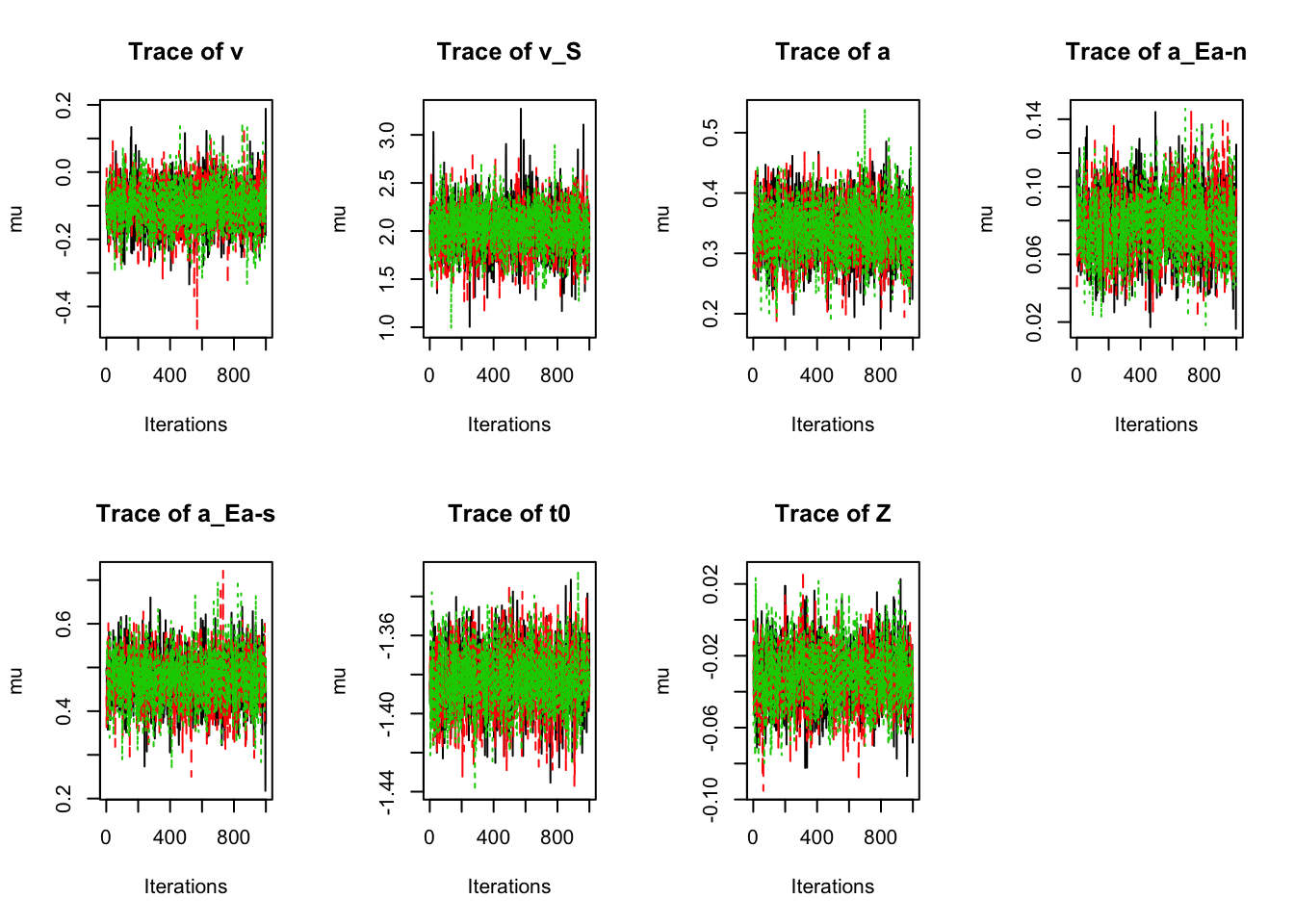
Now let’s check the convergence and efficiency;
round(gd_pmwg(sPNAS_a,selection="mu"),2) ## [1] 1## v v_S a a_Ea-n a_Ea-s t0 Z mpsrf
## 1 1 1 1 1 1 1 1round(es_pmwg(sPNAS_a,selection="mu"))## a_Ea-n Z v t0 a_Ea-s a v_S
## 1596 1921 2404 2458 2731 2793 2886## v v_S a a_Ea-n a_Ea-s t0 Z
## 2404 2886 2793 1596 2731 2458 1921iat_pmwg(sPNAS_a,selection="mu")## v_S a a_Ea-s t0 v Z a_Ea-n
## 1.09 1.10 1.14 1.23 1.29 1.62 1.85We can also print autocorrelation functions for each chain (can also be done for alpha).
par(mfrow=c(3,7))
plot_acfs(sPNAS_a,selection="mu",layout=NULL)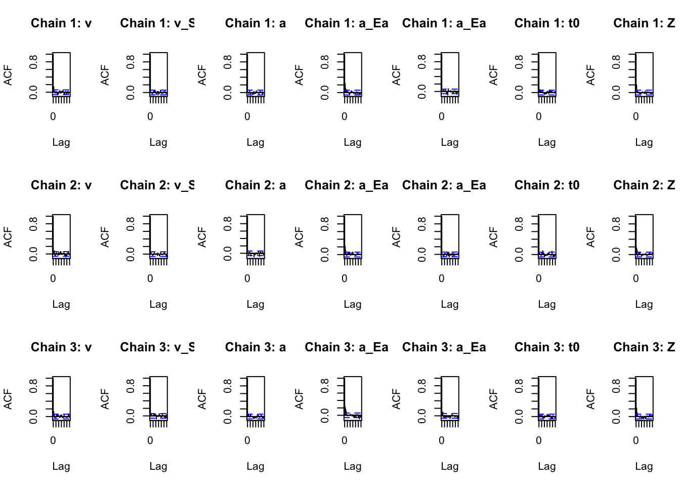
Next, lets check the group level variance;
# Population variance
plot_chains(sPNAS_a,selection="variance",layout=c(2,4))
round(gd_pmwg(sPNAS_a,selection="variance"),2)
## [1] 1.01## v v_S a a_Ea-n a_Ea-s t0 Z mpsrf
## 1.00 1.00 1.00 1.00 1.00 1.00 1.00 1.01round(es_pmwg(sPNAS_a,selection="variance"))## a_Ea-n Z v t0 a a_Ea-s v_S
## 706 846 1125 1608 1915 1984 2372## v v_S a a_Ea-n a_Ea-s t0 Z
## 1125 2372 1915 706 1984 1608 846iat_pmwg(sPNAS_a,selection="variance")## v_S a_Ea-s a t0 v Z a_Ea-n
## 1.29 1.51 1.59 1.76 2.95 3.71 3.91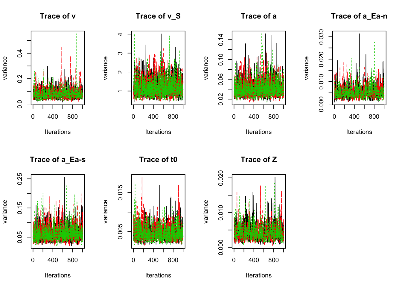
And finally, let’s look at the group level covariance;
# There are p*(p-1)/2 correlations, where p = number of parameters.
plot_chains(sPNAS_a,selection="correlation",layout=c(3,7),ylim=c(-1,1))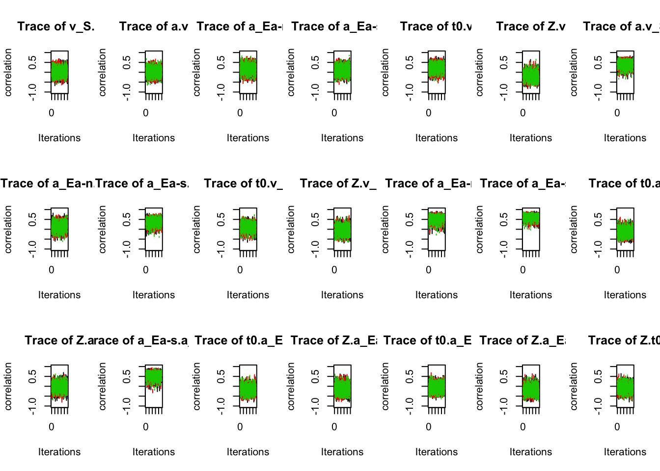
# All are estimated quite well without strong autocorrelation.
round(gd_pmwg(sPNAS_a,selection="correlation"),2)
## [1] 1.01## v_S.v a.v a_Ea-n.v a_Ea-s.v t0.v Z.v
## 1.00 1.00 1.00 1.00 1.00 1.00
## a.v_S a_Ea-n.v_S a_Ea-s.v_S t0.v_S Z.v_S a_Ea-n.a
## 1.00 1.00 1.00 1.00 1.00 1.00
## a_Ea-s.a t0.a Z.a a_Ea-s.a_Ea-n t0.a_Ea-n Z.a_Ea-n
## 1.00 1.00 1.00 1.00 1.00 1.00
## t0.a_Ea-s Z.a_Ea-s Z.t0 mpsrf
## 1.00 1.00 1.00 1.01round(es_pmwg(sPNAS_a,selection="correlation"))## Z.a_Ea-n a_Ea-s.a_Ea-n a_Ea-n.a a_Ea-n.v_S Z.a Z.v
## 1215 1224 1360 1500 1503 1531
## Z.a_Ea-s a_Ea-n.v Z.t0 Z.v_S t0.v t0.a_Ea-n
## 1606 1800 1829 1836 1880 1922
## a_Ea-s.a v_S.v a_Ea-s.v a.v a_Ea-s.v_S a.v_S
## 2012 2199 2222 2260 2285 2725
## t0.v_S t0.a_Ea-s t0.a
## 2729 2770 3356## v_S.v a.v a_Ea-n.v a_Ea-s.v t0.v Z.v
## 2199 2260 1800 2222 1880 1531
## a.v_S a_Ea-n.v_S a_Ea-s.v_S t0.v_S Z.v_S a_Ea-n.a
## 2725 1500 2285 2729 1836 1360
## a_Ea-s.a t0.a Z.a a_Ea-s.a_Ea-n t0.a_Ea-n Z.a_Ea-n
## 2012 3356 1503 1224 1922 1215
## t0.a_Ea-s Z.a_Ea-s Z.t0
## 2770 1606 1829iat_pmwg(sPNAS_a,selection="correlation")## t0.a_Ea-s a.v_S t0.a t0.v_S a_Ea-s.v_S a.v
## 1.16 1.16 1.16 1.18 1.30 1.35
## a_Ea-s.v v_S.v a_Ea-s.a t0.v Z.v_S t0.a_Ea-n
## 1.37 1.41 1.48 1.54 1.64 1.72
## Z.t0 Z.a a_Ea-n.v_S Z.v Z.a_Ea-s a_Ea-n.v
## 1.73 1.83 1.97 1.97 2.04 2.24
## a_Ea-n.a a_Ea-s.a_Ea-n Z.a_Ea-n
## 2.45 2.45 2.515.9 Model Fit
The next important part of model-based sampling is checking the fit of the model. It’s important to remember that no model is perfect, and models are just that - models or representations, so it’s common to observe some misfit. Whilst a perfect fit is not imperative, interpreting the modelling results in the context if the fit is important. For example, if we were to fit 3 models, each with testing a different hypotheses for the same manipulation, we could find a “winning model” that best describes the data (more on this in the model comparison section). However, we need to check the fit of the winning model to contextualise our findings. We may see a significant amount of misfit - in this example, even though the winning model is the best explanation for the data we observed, and it helps us to rule out other hypotheses, it is important to discuss the misfit as other, untested hypotheses or models may explain the data even better.
Assessing the model fit can be tricky, so we provide several functions to graphically observe the model fit. This is done using the plot_fit function. By default the plot shows results for all subjects, putting everyone on the same x scale, which can make it hard to see fit for some or most subjects. The plots shown here are cumulative density plots, which shows RT on the x axis and density on the y axis. These plots are shown for each emphasis condition for both left and right stimuli (i.e., all factors we tested), with left and right responses plotted for both observed (solid line) and model-predicted data (gray line). Generally, this will plot the fit for all subjects. Here we just show one participant;
# plot for a single subject, e.g., the first
plot_fit(dat,ppPNAS_a,layout=c(2,3),subject="as1t")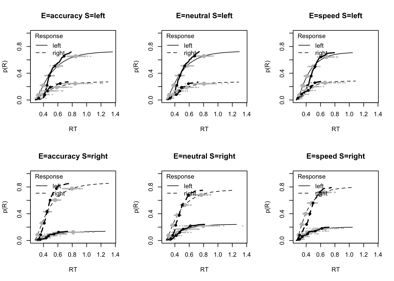
Below are several other examples of fit plots that you can check out;
# Or plot for all subjects
plot_fit(dat,ppPNAS_a,layout=c(2,3))


# You could specify your own limits (e.g,. the data range) and move the legend)
plot_fit(dat,ppPNAS_a,layout=c(2,3),xlim=c(.25,1.5),lpos="right")

# This function (note the "s" in plot_fits) does the x scaling per subject
plot_fits(dat,ppPNAS_a,layout=c(2,3),lpos="right")

# Can also show the average over subjects as subjects is like any other factor,
# so just omit it. We see that the fit is OK but has various misses.
plot_fit(dat,ppPNAS_a,layout=c(2,3),factors=c("E","S"),lpos="right",xlim=c(.25,1.5))
We can also use plot_fit to examine specific aspects of fit by supplying a function that calculates a particular statistic for the data. For example to look at accuracy we might use (where d is a data frame containing the observed data or or posterior predictives) this to get percent correct. Drilling down on accuracy we see the biggest misfit is in speed for right responses by > 5%.
#
pc <- function(d) 100*mean(d$S==d$R)

plot_fit(dat,ppPNAS_a,layout=c(2,3),factors=c("E","S"),
         stat=pc,stat_name="Accuracy (%)",xlim=c(70,95))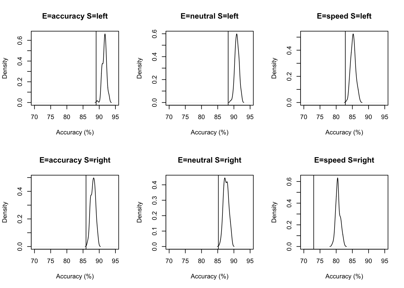
These plots show that the Weiner diffusion model does an okay job of predicting accuracy (it’s in the right direction at least), however, there is clearly some misfit going on here. What might cause this?
Conversely for mean RT the biggest misses are over-estimation of RT by 50ms or more in the accuracy and neutral conditions;
tab <- plot_fit(dat,ppPNAS_a,layout=c(2,3),factors=c("E","S"),
         stat=function(d){mean(d$rt)},stat_name="Mean RT (s)",xlim=c(0.375,.625))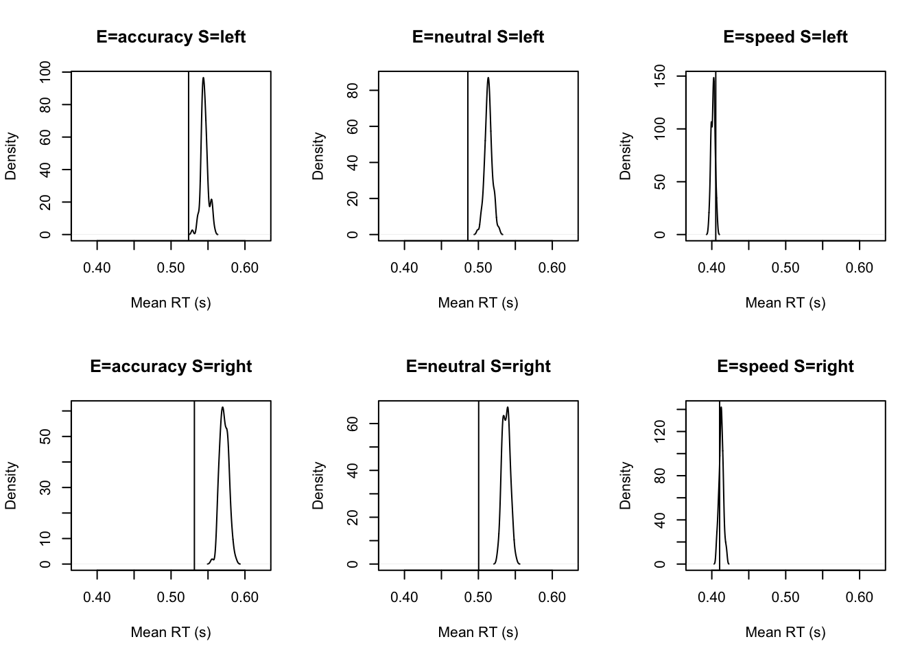
round(tab,2)## Observed 2.5% 50% 97.5%
## E=accuracy S=left 0.52 0.54 0.54 0.56
## E=accuracy S=right 0.53 0.56 0.57 0.58
## E=neutral S=left 0.49 0.50 0.51 0.52
## E=neutral S=right 0.50 0.53 0.54 0.55
## E=speed S=left 0.41 0.40 0.40 0.41
## E=speed S=right 0.41 0.41 0.41 0.42Below, we’ve included several other tests that you can look at to assess the fit of the model. These look at predition of response times for different percentiles, as well as response time variability and speed of errors.
# However for fast responses (10th percentile) there is global under-prediction.
tab <- plot_fit(dat,ppPNAS_a,layout=c(2,3),factors=c("E","S"),xlim=c(0.275,.375),
         stat=function(d){quantile(d$rt,.1)},stat_name="10th Percentile (s)")
round(tab,2)

# and for slow responses (90th percentile) global over-prediction .
tab <- plot_fit(dat,ppPNAS_a,layout=c(2,3),factors=c("E","S"),xlim=c(0.525,.975),
         stat=function(d){quantile(d$rt,.9)},stat_name="90th Percentile (s)")
round(tab,2)

# This corresponds to global under-estimation of RT variability.
tab <- plot_fit(dat,ppPNAS_a,layout=c(2,3),factors=c("E","S"),
         stat=function(d){sd(d$rt)},stat_name="SD (s)",xlim=c(0.1,.355))
round(tab,2)


# Errors tend to be much faster than the models for all conditions.
tab <- plot_fit(dat,ppPNAS_a,layout=c(2,3),factors=c("E","S"),xlim=c(0.375,.725),
         stat=function(d){mean(d$rt[d$R!=d$S])},stat_name="Mean Error RT (s)")
round(tab,2)
5.10 Posterior parameter inference
5.10.1 Means
Making inference is the key step for modelling, as we want to take our models and really delve into the results in relation to our hypotheses. To do this, we can make inference on the posterior parameter estimates. First, let’s look at population mean tests (theta mu). Let’s first look at the credible intervals (95%) for the sampled parameters. These can allow us to see whether an effect was present in difference parameters (i.e., does the estimated parameter cross 0 or not), as well as looking at estimates for the other parameters (on the sampled scale). For this we use plot_density without plotting to get a table of 95% parameter CIs.
ciPNAS <- plot_density(sPNAS_a,layout=c(2,4),selection="mu",do_plot=FALSE)
round(ciPNAS,2)
## v v_S a a_Ea-n a_Ea-s t0 Z
## 2.5% -0.23 1.54 0.25 0.04 0.36 -1.41 -0.06
## 50% -0.10 2.02 0.34 0.08 0.47 -1.38 -0.03
## 97.5% 0.03 2.50 0.43 0.12 0.59 -1.35 0.00We will also do testing of the “mapped” parameters, that is, parameters transformed to the scale used by the model and mapped to the design cells. To illustate here are the mapped posterior medians
mapped_par(ciPNAS[2,],design_a)## S E lR lM v a sv t0 st0 s Z SZ DP z sz d
## 1 left accuracy left TRUE -2.123 1.401 0 0.251 0 1 0.487 0 0.5 0.682 0 0
## 2 left neutral left TRUE -2.123 1.296 0 0.251 0 1 0.487 0 0.5 0.631 0 0
## 3 left speed left TRUE -2.123 0.875 0 0.251 0 1 0.487 0 0.5 0.427 0 0
## 4 right accuracy left TRUE 1.925 1.401 0 0.251 0 1 0.487 0 0.5 0.682 0 0
## 5 right neutral left TRUE 1.925 1.296 0 0.251 0 1 0.487 0 0.5 0.631 0 0
## 6 right speed left TRUE 1.925 0.875 0 0.251 0 1 0.487 0 0.5 0.427 0 05.10.1.1 Visualising results
Now we’re going to show some extensions of visualizations, by first extracting the parameter estimates, and then plotting these using ggplot2. Let’s start by extracting the parameters and checking the means of the posterior.
Here you might want to use the CI/mapped_par tables to visualize certain parameter effects. Here we plot median thresholds with 95% CIs for each emphasis condition (we will test for statistically significant differences next).
library(tidyverse)

# Get CIs from plot_density
# ciPNAS <- plot_density(sPNAS_a,layout=c(2,4),selection="mu",do_plot=FALSE)
# round(ciPNAS,2)

# Pull out medians, lower and upper CIs in long format for ggplot
# Note thresholds are the same for S=left/right so here we only keep rows 1-3
# of the mapped_par table. This is not essential, since ggplot plot would plot
# the (identical) values for left/right on top of each other, still giving the
# desired result visually.
plot_df <- data.frame(
  mapped_par(ciPNAS[2,],design_a)[1:3,c("E","a")],  # 0.5 quantile
  lower = mapped_par(ciPNAS[1,],design_a)[1:3,c("a")],  # 0.025 quantile
  upper = mapped_par(ciPNAS[3,],design_a)[1:3,c("a")]  # 0.975 quantile
)
plot_df
## E a lower upper
## 1 accuracy 1.401 1.284 1.531
## 2 neutral 1.296 1.232 1.364
## 3 speed 0.875 0.897 0.853Now we can plot thresholds
a_plot <- ggplot(data = plot_df, aes(E, a)) +
  geom_line(aes(group = 1), lty = "dashed", lwd = 1, alpha = 0.5) +
  geom_point(size = 4, shape = 19) +
  geom_errorbar(aes(ymax = upper, ymin = lower, width = 0.4)) +
  ylim(0.6, 1.6) + xlab("Emphasis") +
  theme_minimal() + theme(text = element_text(size = 15))
a_plot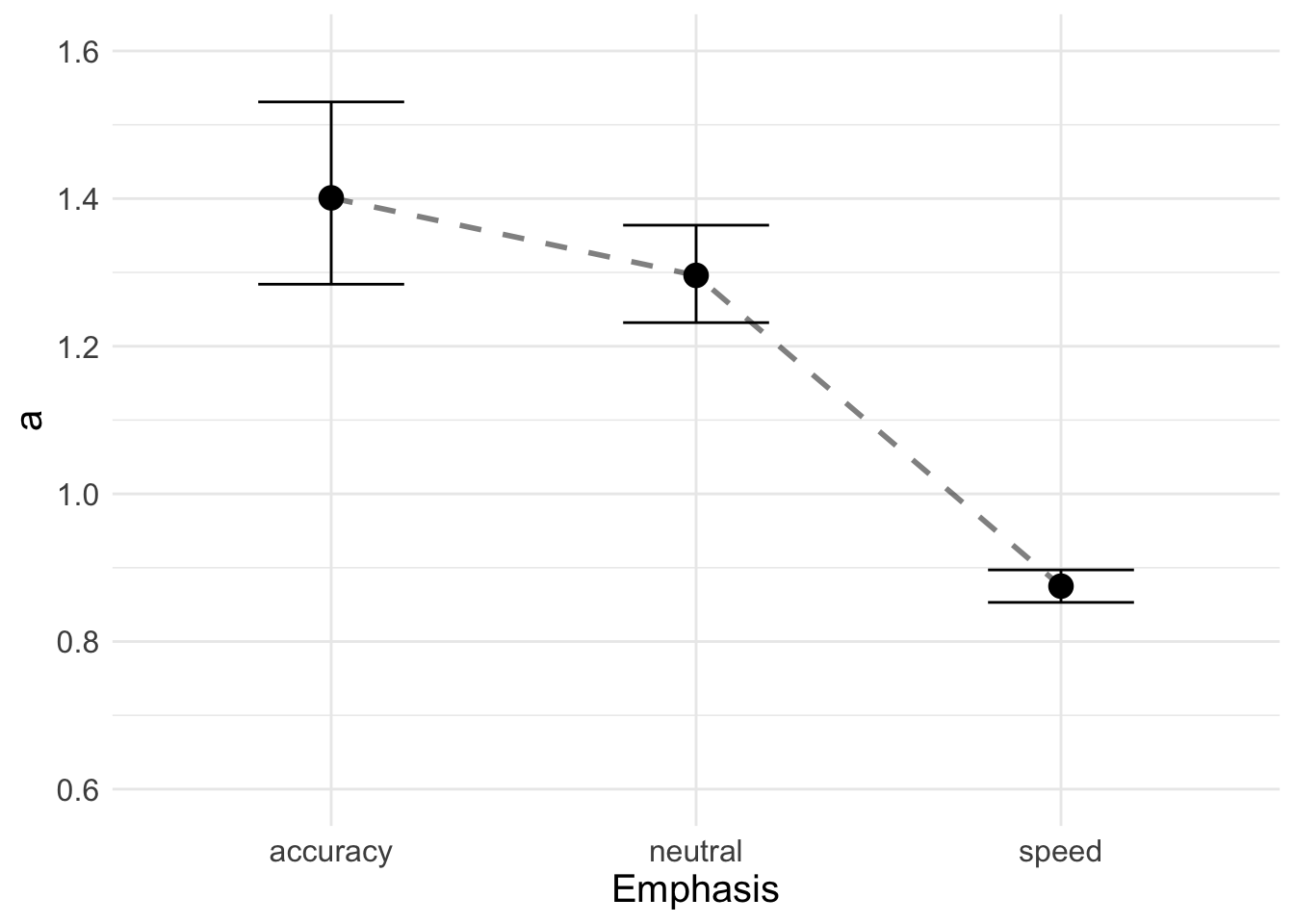
Note that for plotting difference effects or interactions, you can perform the relevant calculations on the samples contained in parameters_data_frame
head(parameters_data_frame(sPNAS_a, mapped = TRUE))## v_left v_right a_accuracy a_neutral a_speed t0 Z
## 1 -2.135403 1.995592 1.403917 1.257892 0.8586231 0.2506575 0.4885954
## 2 -1.823649 1.735639 1.441444 1.311179 0.8760923 0.2477816 0.4879099
## 3 -2.434109 2.147717 1.365601 1.253614 0.8479388 0.2487847 0.4827206
## 4 -2.326312 1.998673 1.376405 1.275819 0.8997932 0.2552087 0.4946387
## 5 -2.030125 1.779503 1.357193 1.264123 0.8840312 0.2516569 0.4931881
## 6 -2.329081 2.013524 1.421591 1.304193 0.8562077 0.2502680 0.48972425.10.2 Inference
Testing can be performed with the p_test function, which is similar to the base R t.test function. By default its assumes selection=“mu”. If just one “x” is specified it tests whether a single parameter differs from zero, reproducing one of the credible intervals in the table above, but with the probability of being less than zero.
Let’s first look at rates from the estimated DDM;
p_test(x=sPNAS_a,x_name="v")## v mu
## 2.5% -0.23 NA
## 50% -0.10 0
## 97.5% 0.03 NA
## attr(,"less")
## [1] 0.94There is a slight drift-rate bias to left (lower) but not credible at 95%.
p_test(x=sPNAS_a,x_name="v",alternative = "greater")## v mu
## 2.5% -0.23 NA
## 50% -0.10 0
## 97.5% 0.03 NA
## attr(,"greater")
## [1] 0.06In this case it might be better to get the probability of greater than zero.
p_test(sPNAS_a,x_name="v_S")## v_S mu
## 2.5% 1.54 NA
## 50% 2.02 0
## 97.5% 2.50 NA
## attr(,"less")
## [1] 0The main effect of stimulus (i.e., the conventional DDM drift rate) is clearly greater than zero.
Now let’s look at other parameters. You can try these all for yourself!
## Non-decision time

# Recall non-decision time is on a log scale
p_test(sPNAS_a,x_name="t0")
# We can also test transformed parameters by specifying a function. The x_name
# is just used in the table header.
p_test(sPNAS_a,x_fun=function(x){exp(x["t0"])},x_name="t0(sec)")
# Alternatively p_test can automatically transform to the scale used by the
# model, here producing the same result.
p_test(x=sPNAS_a,x_name="t0",mapped=TRUE)

## Start-point bias

# Here we both transform and then test again the unbiased level (0.5). There is
# a very close to (two tailed 95%) credible bias to left (lower), to get more
# resolution we up the default digits.
p_test(sPNAS_a,x_name="Z",x_fun=function(x){pnorm(x["Z"])},
       mu=0.5,digits=4,alternative = "greater")

## Threshold

# Transforming thresholds to the natural scale
p_test(sPNAS_a,x_name="a",x_fun=function(x){exp(x["a"])})
# Accuracy threshold is credibly but not much greater than neutral
p_test(sPNAS_a,x_name="a_Ea-n")
# Accuracy threshold is much greater than speed.
p_test(sPNAS_a,x_name="a_Ea-s")
5.10.3 Mapped
Using the mapped=TRUE argument not only transforms to the scale used by the model but also to the cells of the design, automatically generating appropriate names which can be seen using this function, where for example, we could test if the threshold for speed differs from zero
p_names(sPNAS_a,mapped=TRUE)$a## [1] "a_accuracy" "a_neutral" "a_speed"p_test(x=sPNAS_a,x_name="a_speed",mapped=TRUE)## a_speed mu
## 2.5% 0.80 NA
## 50% 0.88 0
## 97.5% 0.96 NA
## attr(,"less")
## [1] 0mapped=TRUE also allows arbitrary comparisons between cells to be done. For example, we can compare the difference between neutral and speed.
p_test(x=sPNAS_a,x_name="n-s",mapped=TRUE,x_fun=function(x){diff(x[c("a_speed","a_neutral")])})## n-s mu
## 2.5% 0.31 NA
## 50% 0.42 0
## 97.5% 0.53 NA
## attr(,"less")
## [1] 0The same thing can be achieved by specifying and x and y argument;
p_test(x=sPNAS_a,x_name="a_neutral",y=sPNAS_a,y_name="a_speed",mapped=TRUE)## a_neutral a_speed a_neutral-a_speed
## 2.5% 1.2 0.80 0.31
## 50% 1.3 0.88 0.42
## 97.5% 1.4 0.96 0.53
## attr(,"less")
## [1] 0More generally we can test differences between combinations of cells using a function. For example, is the average of accuracy and neutral different from speed?
p_test(x=sPNAS_a,x_name="an-s",mapped=TRUE,x_fun=function(x){
  sum(x[c("a_accuracy","a_neutral")])/2 - x["a_speed"]})
## an-s mu
## 2.5% 0.36 NA
## 50% 0.47 0
## 97.5% 0.59 NA
## attr(,"less")
## [1] 05.10.4 Variability
Next lets assess population variability. Here we cannot use mapping, as these parameters are about variability on the sampled scale, but we can still make tests.
ciPNAS <- plot_density(sPNAS_a,layout=c(2,4),selection="variance",do_plot=FALSE)
round(ciPNAS,3)
## v v_S a a_Ea-n a_Ea-s t0 Z
## 2.5% 0.033 0.580 0.021 0.002 0.030 0.002 0.001
## 50% 0.071 1.080 0.038 0.004 0.056 0.004 0.004
## 97.5% 0.173 2.256 0.079 0.012 0.121 0.009 0.009Suppose we wanted to compare standard deviations of the accuracy-neutral and accuracy minus speed contrasts;
p_test(x=sPNAS_a,x_name="a_Ea-n",x_fun=function(x){sqrt(x["a_Ea-s"])},
  y=sPNAS_a,y_name="a_Ea-s",y_fun=function(x){sqrt(x["a_Ea-n"])},selection="variance")
## a_Ea-n a_Ea-s a_Ea-n-a_Ea-s
## 2.5% 0.17 0.04 0.10
## 50% 0.24 0.07 0.17
## 97.5% 0.35 0.11 0.27
## attr(,"less")
## [1] 05.10.5 Covariance/correlations
Another interesting metric to asses is population correlation. Again mapped can’t be tested for the same reason as above. There are lots of these so lets look at them first overall.
ciPNAS <- plot_density(sPNAS_a,layout=c(2,4),selection="correlation",do_plot=FALSE)
round(ciPNAS,3)
## v_S.v a.v a_Ea-n.v a_Ea-s.v t0.v Z.v a.v_S a_Ea-n.v_S a_Ea-s.v_S
## 2.5% -0.422 -0.416 -0.296 -0.338 -0.235 -0.654 -0.022 -0.338 -0.063
## 50% 0.035 0.039 0.214 0.122 0.246 -0.241 0.424 0.170 0.388
## 97.5% 0.486 0.477 0.644 0.555 0.625 0.259 0.718 0.599 0.700
## t0.v_S Z.v_S a_Ea-n.a a_Ea-s.a t0.a Z.a a_Ea-s.a_Ea-n t0.a_Ea-n Z.a_Ea-n
## 2.5% -0.359 -0.499 0.100 0.257 -0.549 -0.496 0.114 -0.607 -0.615
## 50% 0.080 -0.047 0.561 0.640 -0.154 -0.030 0.594 -0.195 -0.155
## 97.5% 0.491 0.411 0.821 0.847 0.302 0.425 0.844 0.271 0.373
## t0.a_Ea-s Z.a_Ea-s Z.t0
## 2.5% -0.487 -0.641 -0.540
## 50% -0.067 -0.227 -0.111
## 97.5% 0.375 0.299 0.374The strongest correlations are among the a parameters. Do the two intercept-effect correlations differ?
p_test(x=sPNAS_a,x_name="a_Ea-n.a",y=sPNAS_a,y_name="a_Ea-s.a",selection="correlation")## a_Ea-n.a a_Ea-s.a a_Ea-n.a-a_Ea-s.a
## 2.5% 0.10 0.26 -0.50
## 50% 0.56 0.64 -0.07
## 97.5% 0.82 0.85 0.27
## attr(,"less")
## [1] 0.673Here, their imprecise estimation makes any difference not credible.
It is also important to note that the intercept and effect contrasts are themselves not orthogonal, which will induce a correlation. This can be seen from the dot products of their design matrix being non-zero. The two effects are orthogonal so this is not a factor in their positive correlation.
get_design_matrix(sPNAS_a)$a## a a_Ea-n a_Ea-s
## 1 1 0 0
## 39 1 -1 0
## 77 1 0 -1p_test(sPNAS_a,x_name="a_Ea-s.a_Ea-n",selection="correlation")## a_Ea-s.a_Ea-n mu
## 2.5% 0.11 NA
## 50% 0.59 0
## 97.5% 0.84 NA
## attr(,"less")
## [1] 0.009Otherwise the table above reveals no credible correlations.
5.10.6 Random effect (alpha) tests
We can test individual participants, with the first one selected by default.
p_test(x=sPNAS_a,x_fun=function(x){exp(x["t0"])},x_name="t0(sec)",
selection="alpha",digits=3)## Testing x subject as1t## t0(sec) mu
## 2.5% 0.240 NA
## 50% 0.243 0
## 97.5% 0.246 NA
## attr(,"less")
## [1] 0We can also compare two participants, for example bd6t has slightly but credibly slower non-decision time than as1t.
snams <- subject_names(sPNAS_a)
p_test(selection="alpha",digits=3,
x=sPNAS_a,x_fun=function(x){exp(x["t0"])},x_name="t0(s)",x_subject=snams[2],
y=sPNAS_a,y_fun=function(x){exp(x["t0"])},y_name="t0(s)",y_subject=snams[1])## Testing x subject bd6t## Testing y subject as1t## t0(s)_bd6t t0(s)_as1t bd6t-as1t
## 2.5% 0.248 0.240 0.003
## 50% 0.250 0.243 0.007
## 97.5% 0.253 0.246 0.011
## attr(,"less")
## [1] 0# Once again we can use mapping to the same effect
p_test(selection="alpha",digits=3,mapped=TRUE,
x=sPNAS_a,x_name="t0",x_subject=snams[2],
y=sPNAS_a,y_name="t0",y_subject=snams[1])## Testing x subject bd6t
## Testing y subject as1t## t0_bd6t t0_as1t bd6t-as1t
## 2.5% 0.248 0.240 0.003
## 50% 0.250 0.243 0.007
## 97.5% 0.253 0.246 0.011
## attr(,"less")
## [1] 05.10.7 Extracting a data frame of parameters
Parameters can be extracted into a data frame for further analysis, by default getting mu from the sample stage. Here we could also include contrasts, mapped parameters and/or random effects. Here we only show the output for one of these (default), but code is included for all examples mentioned.
## v v_S a a_Ea-n a_Ea-s t0 Z
## 1 -0.06990526 2.065498 0.3392660 0.10982898 0.4916912 -1.383668 -0.02859105
## 2 -0.04400465 1.779644 0.3656451 0.09471846 0.4979289 -1.395208 -0.03030996
## 3 -0.14319610 2.290913 0.3115943 0.08556377 0.4765411 -1.391167 -0.04332662
## 4 -0.16381979 2.162492 0.3194753 0.07588717 0.4250656 -1.365674 -0.01343924
## 5 -0.12531054 1.904814 0.3054189 0.07104042 0.4286819 -1.379689 -0.01707575
## 6 -0.15777829 2.171303 0.3517766 0.08619187 0.5070189 -1.385223 -0.02576044head(parameters_data_frame(sPNAS_a))
# If desired constants can be included
head(parameters_data_frame(sPNAS_a,include_constants=TRUE))
# Or mapped parameters
head(parameters_data_frame(sPNAS_a,mapped=TRUE))
# If random effects are selected a subjects factor column is added
head(parameters_data_frame(sPNAS_a,selection="alpha",mapped=TRUE))5.10.7.1 Visualisations
Here we plot thresholds using the samples extracted from the parameter_data_frame function
# Get data frame with all 3000 sampling iterations for each parameter
ps <- parameters_data_frame(sPNAS_a,mapped=TRUE)
head(ps)## v_left v_right a_accuracy a_neutral a_speed t0 Z
## 1 -2.135403 1.995592 1.403917 1.257892 0.8586231 0.2506575 0.4885954
## 2 -1.823649 1.735639 1.441444 1.311179 0.8760923 0.2477816 0.4879099
## 3 -2.434109 2.147717 1.365601 1.253614 0.8479388 0.2487847 0.4827206
## 4 -2.326312 1.998673 1.376405 1.275819 0.8997932 0.2552087 0.4946387
## 5 -2.030125 1.779503 1.357193 1.264123 0.8840312 0.2516569 0.4931881
## 6 -2.329081 2.013524 1.421591 1.304193 0.8562077 0.2502680 0.4897242We will just plot means for now. For an optional exercise, see if you can add error bars to the plots below (e.g., 95% CIs, standard deviation, etc.)
pmeans <- data.frame(lapply(ps, mean))
pmeans## v_left v_right a_accuracy a_neutral a_speed t0 Z
## 1 -2.122904 1.922171 1.403018 1.297817 0.8763915 0.2508947 0.4872616# Put into a nicely labelled long format data frame for ggplot
a <- pmeans %>% transmute(Accuracy = a_accuracy,
Neutral = a_neutral,
Speed = a_speed) %>%
pivot_longer(cols = everything(),
names_to = c("Emphasis"),
names_pattern = "(.*)",
values_to = "a")
a## # A tibble: 3 x 2
## Emphasis a
## <chr> <dbl>
## 1 Accuracy 1.40
## 2 Neutral 1.30
## 3 Speed 0.876Now we can also plot thresholds;
a_plot <- ggplot(data = a, aes(Emphasis, a)) +
geom_line(aes(group = 1), lty = "dashed", lwd = 1, alpha = 0.5) +
geom_point(size = 4, shape = 19) +
ylim(0.6, 1.6) +
theme_minimal() + theme(text = element_text(size = 15))
a_plot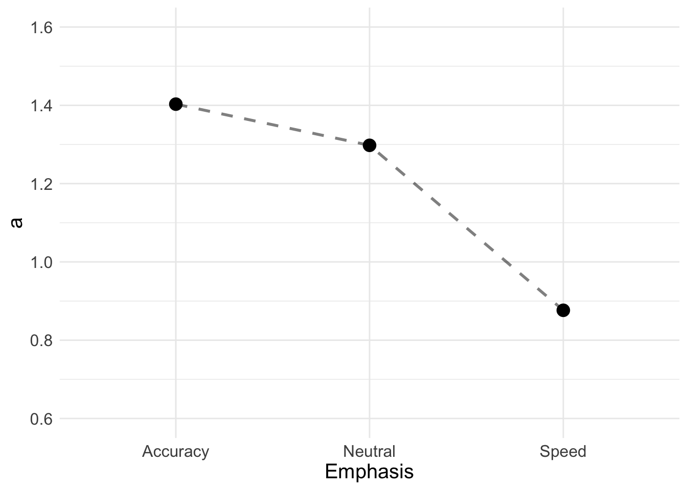
5.11 FULL DDM
Once trial-to-trial variability parameters are estimated the sampler can sometimes explore regions where the numerical approximation to the DDM’s likelihood become inaccurate. In order to avoid this log_likelihood_ddm (in emc/likelihood.R) imposes the following restrictions on these parameters (we also restrict v and a to typical regions), returning low likelihoods when they are violated.
abs(v)<5 | a<2 | sv<2 | sv>.1 | SZ<.75 | SZ>.01 | st0<.2
These are usually appropriate for the seconds scale with s=1 fixed. For some data and/or different scalings they may have to be adjusted. Posterior estimates should be checked to see if estimates are stacking up against these bounds, indicating they might need adjustment. Alternatively, poor convergence behaviour may indicate the need for further restriction.
load("~/Desktop/emc2/models/DDM/DDM/examples/samples/sPNAS_a_full.RData")Lets now fit the full DDM analogous to the Wiener model fit previously.
design_a_full <- make_design(
Ffactors=list(subjects=levels(dat$subjects),S=levels(dat$S),E=levels(dat$E)),
Rlevels=levels(dat$R),
Clist=list(S=Vmat,E=Emat),
Flist=list(v~S,a~E,sv~1, t0~1, st0~1, s~1, Z~1, SZ~1, DP~1),
constants=c(s=log(1),DP=qnorm(0.5)),
model=ddmTZD)
samplers <- make_samplers(dat,design_a_full,type="standard")
save(samplers,file="sPNAS_a_full.RData")## v v_S a a_Ea-n a_Ea-s sv t0 st0 Z SZ
## 0 0 0 0 0 0 0 0 0 0
## attr(,"map")
## attr(,"map")$v
## v v_S
## 1 1 -1
## 20 1 1
##
## attr(,"map")$a
##    a a_Ea-n a_Ea-s
## 1  1      0      0
## 39 1     -1      0
## 77 1      0     -1
##
## attr(,"map")$sv
## sv
## 1 1
##
## attr(,"map")$t0
## t0
## 1 1
##
## attr(,"map")$st0
## st0
## 1 1
##
## attr(,"map")$s
## s
## 1 1
##
## attr(,"map")$Z
## Z
## 1 1
##
## attr(,"map")$SZ
## SZ
## 1 1
##
## attr(,"map")$DP
## DP
## 1 15.11.1 Estimating the model
To estimate the model, we use the code below. This may take longer than the Weiner diffusion, as it is more difficult to estimate.
Note Running this code will take a significant amount of computer power (6 cpus) and may take several minutes-hours depending on the computer. We recommend sourcing the supplied examples if you are following along with the code. This can be done by saving the samples from OSF to your desktop and using; load("Desktop/osfstorage-archive/DDM/sPNAS_a_full.RData")
rm(list=ls())
source("emc/emc.R")
source("models/DDM/DDM/ddmTZD.R")
sPNAS_a_full <- run_burn(sPNAS_a_full,cores_per_chain=7)
save(sPNAS_a_full,file="sPNAS_a_full.RData")
sPNAS_a_full <- run_adapt(sPNAS_a_full,cores_per_chain=7)
save(sPNAS_a_full,file="sPNAS_a_full.RData")
sPNAS_a_full <- run_sample(sPNAS_a_full,iter=1000,cores_per_chain=7)
save(sPNAS_a_full,file="sPNAS_a_full.RData")
ppPNAS_a_full <- post_predict(sPNAS_a_full,n_cores=19)
save(ppPNAS_a_full,sPNAS_a_full,file="sPNAS_a_full.RData")5.11.2 Outcomes
The following code goes through similar steps as we tried earlier for the Weiner diffusion model. We include code below, but only focus on a few specific elements. First, lets load the samples.
load("~/Desktop/emc2/models/DDM/DDM/examples/samples/sPNAS_a_full.RData")We can then check our fitting and convergence metrics. Below, we only run one of these functions to exemplify some misfit, however, it’s important to try these functions for yourself and check the performance and behaviour of the model.
chain_n(sPNAS_a_full)
plot_chains(sPNAS_a_full,layout=c(3,7),selection="LL")
# random effects
plot_chains(sPNAS_a_full,layout=c(2,5))
print(round(gd_pmwg(sPNAS_a_full),2))
# As is usual sv and particularly SZ are least efficient
iat_pmwg(sPNAS_a_full)
es_pmwg(sPNAS_a_full,summary=min)
# Same for hyper mean
plot_chains(sPNAS_a_full,layout=c(2,5),selection="mu")
print(round(gd_pmwg(sPNAS_a_full,selection="mu"),2))
iat_pmwg(sPNAS_a_full,selection="mu")
es_pmwg(sPNAS_a_full,selection="mu",summary=min)
# variance
plot_chains(sPNAS_a_full,layout=c(2,5),selection="variance")
print(round(gd_pmwg(sPNAS_a_full,selection="variance"),2))
iat_pmwg(sPNAS_a_full,selection="variance")
es_pmwg(sPNAS_a_full,selection="variance",summary=min)
# and correlation
plot_chains(sPNAS_a_full,layout=c(3,5),selection="correlation")
print(round(gd_pmwg(sPNAS_a_full,selection="correlation"),2))
iat_pmwg(sPNAS_a_full,selection="correlation")
es_pmwg(sPNAS_a_full,selection="correlation",summary=min)plot_chains(sPNAS_a_full,layout=c(2,5),selection="mu")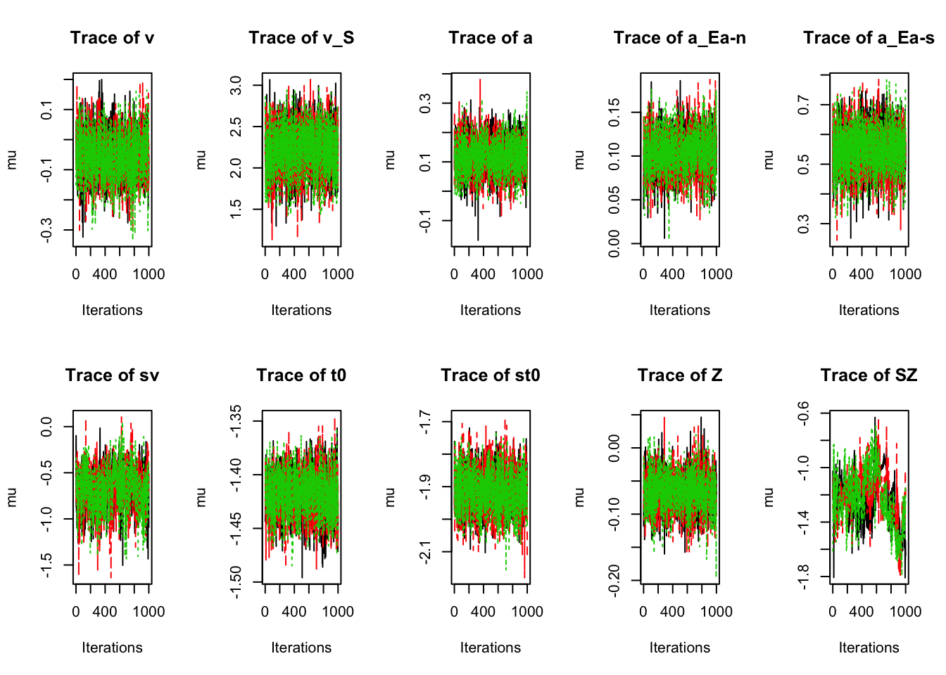 Clearly, there is a lot of noise around
 SZ. If we wished to do inference with SZ we should get more samples. To do this, we can run run_sample for many more iterations.
The code below will look at the model fit. Again, for brevity, we only show one of these generated plots;
# Individual fits - these are improved over the Wiener model
plot_fit(dat,ppPNAS_a_full,layout=c(2,3))
# Average over subjects - these show very clear improvement
plot_fit(dat,ppPNAS_a_full,layout=c(2,3),factors=c("E","S"),lpos="right",xlim=c(.25,1.5))
# Accuracy - misfit is much reduced, although it is still present
# for speed for right responses. This suggests a model with Z~E may be warranted.
pc <- function(d) 100*mean(d$S==d$R)
plot_fit(dat,ppPNAS_a_full,layout=c(2,3),factors=c("E","S"),
stat=pc,stat_name="Accuracy (%)",xlim=c(70,95))
# Mean RT - seems to be well estimated.
tab <- plot_fit(dat,ppPNAS_a_full,layout=c(2,3),factors=c("E","S"),
stat=function(d){mean(d$rt)},stat_name="Mean RT (s)",xlim=c(0.375,.625))
# However for fast responses (10th percentile) under-prediction remains except for speed.
tab <- plot_fit(dat,ppPNAS_a_full,layout=c(2,3),factors=c("E","S"),xlim=c(0.275,.375),
stat=function(d){quantile(d$rt,.1)},stat_name="10th Percentile (s)")
# and for slow responses (90th percentile) clear over-prediction except for speed.
tab <- plot_fit(dat,ppPNAS_a_full,layout=c(2,3),factors=c("E","S"),xlim=c(0.525,.975),
stat=function(d){quantile(d$rt,.9)},stat_name="90th Percentile (s)")
round(tab,2)
# This corresponds to under-estimation of RT variability for speed and
# otherwise over-estimation.
tab <- plot_fit(dat,ppPNAS_a_full,layout=c(2,3),factors=c("E","S"),
stat=function(d){sd(d$rt)},stat_name="SD (s)",xlim=c(0.1,.355))
# Error speed is well estimated except for speed where it is over-estimated.
tab <- plot_fit(dat,ppPNAS_a_full,layout=c(2,3),factors=c("E","S"),xlim=c(0.375,.725),
stat=function(d){mean(d$rt[d$R!=d$S])},stat_name="Mean Error RT (s)")The plot below shows a clear improvement in the model prediction for accuracy compared to the weiner diffusion model. This is a good improvement for our model!
plot_fit(dat,ppPNAS_a_full,layout=c(2,3),factors=c("E","S"),lpos="right",xlim=c(.25,1.5))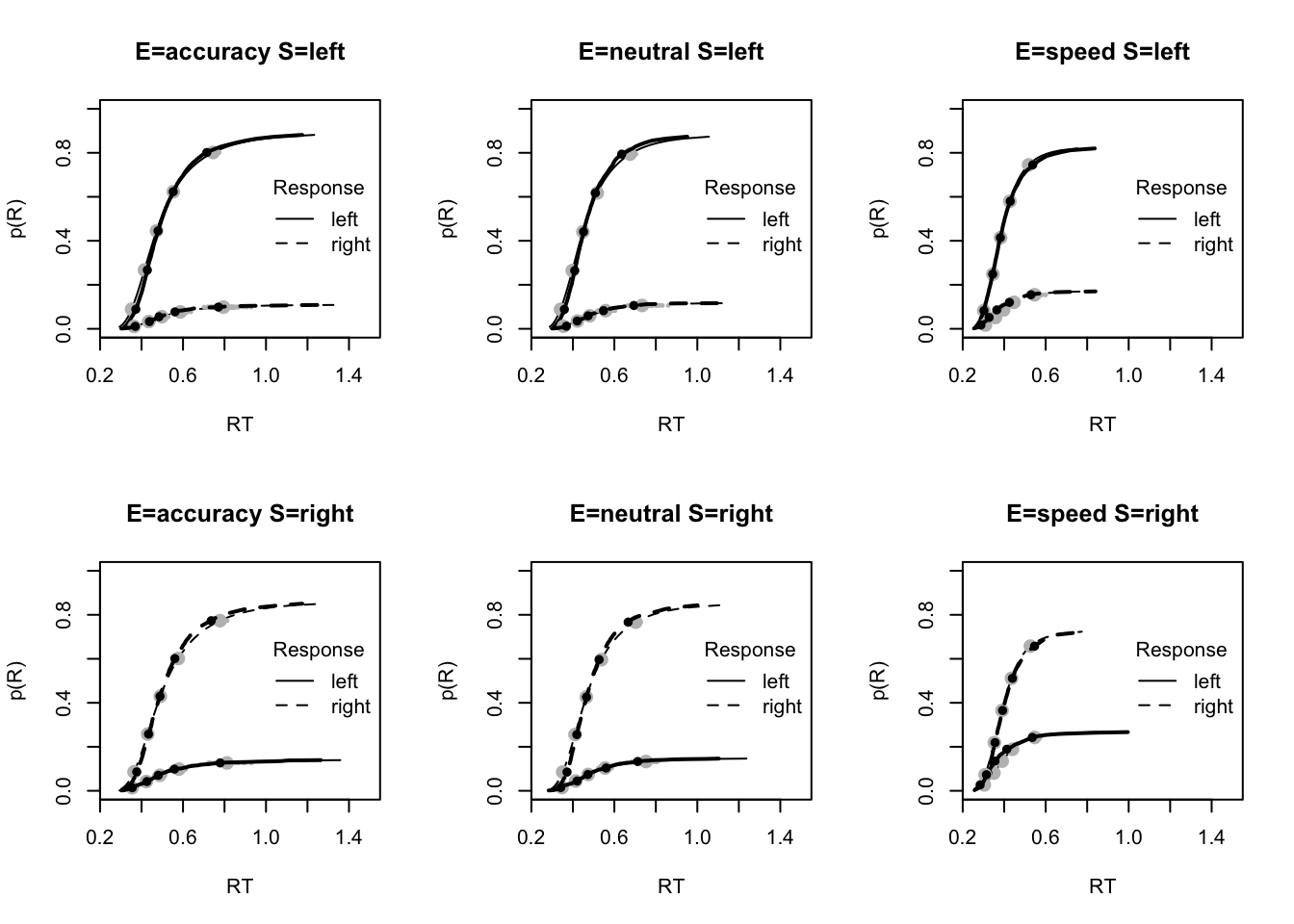
Looking at inference from the model, we can again use plot_density and p_test functions. The code below will perform a variety of relevant inferential tests.
### Population mean (mu) tests
# Priors are dominated, even for sv and SZ
ciPNAS_full <- plot_density(sPNAS_a_full,layout=c(2,5),selection="mu")
# Comparing with the Wiener we see higher rates and overall reduced thresholds
round(ciPNAS_full,2)
round(ciPNAS,2)
# Priors also clearly dominated in mapped parameters
ciPNAS_full_mapped <- plot_density(sPNAS_a_full,layout=c(2,5),selection="mu",mapped=TRUE)
## Rates
# There is a slight drift-rate bias to left (lower) but not credible at 95%
p_test(x=sPNAS_a_full,x_name="v")
# The main effect of stimulus is clearly greater than zero.
p_test(sPNAS_a_full,x_name="v_left",mapped=TRUE)
p_test(sPNAS_a_full,x_name="v_right",mapped=TRUE)
# Rate variability is quite substantial (>20% of the mean)
p_test(x=sPNAS_a_full,x_name="sv",mapped=TRUE)
## Non-decision time
# t0 is now a lower bound so slightly less than in Wiener
p_test(x=sPNAS_a_full,x_name="t0",mapped=TRUE)
# Variability is quite substantial
p_test(x=sPNAS_a_full,x_name="st0",mapped=TRUE)
## Start-point bias
# Small lower (left) bias
p_test(x=sPNAS_a_full,x_name="Z",mapped=TRUE)
# Small level of start-point variability (sz/2 is 11% of .47, i.e., sz = 0.1)
p_test(x=sPNAS_a_full,x_name="SZ",mapped=TRUE)
## Threshold
# Although the overall threshold is reduced the effects are a bit bigger
p_test(sPNAS_a_full,x_name="a",x_fun=function(x){exp(x["a"])})
p_test(sPNAS_a_full,x_name="a_Ea-n")
p_test(sPNAS_a_full,x_name="a_Ea-s")
# For example we could test if the threshold for speed differs from zero
p_test(x=sPNAS_a_full,x_name="a_speed",mapped=TRUE)
# difference between neutral and speed.
p_test(x=sPNAS_a_full,x_name="n-s",mapped=TRUE,x_fun=function(x){
diff(x[c("a_speed","a_neutral")])})
# Average of accuracy and neutral vs. speed
p_test(x=sPNAS_a_full,x_name="an-s",mapped=TRUE,x_fun=function(x){
sum(x[c("a_accuracy","a_neutral")])/2 - x["a_speed"]})
### Variance/correlation
ciPNAS <- plot_density(sPNAS_a_full,layout=c(2,4),selection="variance",do_plot=FALSE)
round(ciPNAS,3)
ciPNAS <- plot_density(sPNAS_a_full,layout=c(2,4),selection="correlation",do_plot=FALSE)
round(ciPNAS,3)5.11.2.1 Visualisations
Here we make a plot comparing thresholds for the Weiner diffusion and full DDM models.
# Get parameter data frame
ps <- parameters_data_frame(sPNAS_a_full,mapped=TRUE)
head(ps)## v_left v_right a_accuracy a_neutral a_speed sv t0 st0
## 1 -2.472714 2.315410 1.131344 1.0872215 0.7301727 0.7789519 0.2360909 0.1398351
## 2 -2.157951 2.142815 1.095963 1.0323258 0.6976620 0.9071532 0.2372373 0.1390481
## 3 -2.062661 2.175118 1.075505 0.9741245 0.6217588 0.4213148 0.2402452 0.1719140
## 4 -2.384422 2.395258 1.211940 1.0962363 0.6585287 0.4628511 0.2402465 0.1438820
## 5 -2.256972 2.256196 1.126258 1.0117172 0.6241981 0.4413305 0.2430235 0.1422897
## 6 -2.022967 2.041279 1.081966 0.9714804 0.6078302 0.4326847 0.2394119 0.1530558
## Z SZ
## 1 0.4636637 0.1467588
## 2 0.4530734 0.1525040
## 3 0.4625686 0.1082340
## 4 0.4711802 0.1190287
## 5 0.4581518 0.1320615
## 6 0.4913602 0.1271238First we can calculate means (or other statistics);
pmeans <- data.frame(lapply(ps, mean))
pmeans
## v_left v_right a_accuracy a_neutral a_speed sv t0 st0
## 1 -2.275758 2.172642 1.129688 1.018313 0.6528586 0.5187465 0.2421431 0.1475707
## Z SZ
## 1 0.4732063 0.1133962Make nicely labelled long format;
a_full <- pmeans %>% transmute(Accuracy = a_accuracy,
                               Neutral = a_neutral,
                               Speed = a_speed) %>%
  pivot_longer(cols = everything(),
               names_to = c("Emphasis"),
               names_pattern = "(.*)",
               values_to = "a")
a_full
## # A tibble: 3 x 2
## Emphasis a
## <chr> <dbl>
## 1 Accuracy 1.13
## 2 Neutral 1.02
## 3 Speed 0.653Now we can make the plot. Full DDM (black) gives lower overall threshold estimates than the Weiner diffusion (grey).
a_plot <- ggplot(data = a_full, aes(Emphasis, a)) +
  geom_line(aes(group = 1), lty = "dashed", lwd = 1, alpha = 0.5) +
  geom_point(size = 4, shape = 19) +
  geom_line(data = a, aes(group = 1), lty = "dashed", lwd = 1, col = "darkgrey") +
  geom_point(data = a, size = 4, shape = 19, col = "darkgrey") +
  ylim(0.4, 1.6) +
  theme_minimal() + theme(text = element_text(size = 15))
a_plot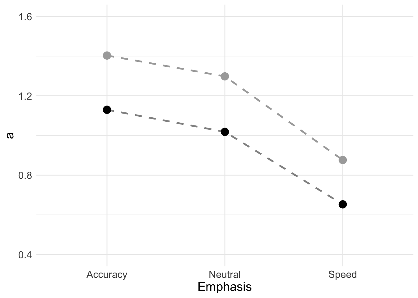
5.12 Parameter recovery study
Next, we’re going to conduct a quick parameter recovery study using the full DDM. We’ll go into more details about the specifics of parameter recovery in following chapters. In this example, we’ll simulate some data given the current data structure that we have. We do this because we want to be sure that the model we’re estimating is able to recover the generating parameters (when we know the true generating values). If we can’t recover the model, this poses a problem for our inference.
To start, we need to create a single simulated data set from that alpha means.
load("~/Desktop/emc2/models/DDM/DDM/examples/samples/sPNAS_a_full.RData")

new_dat <- post_predict(sPNAS_a_full,use_par="mean",n_post=1)
## .Here, we use the parameter values that we estimated in the full PNAS model fit, so these are our “known” values. Now let’s look at whether we can recover these. For simulation and recovery exercises, these can also be useful to establish how many trials and subjects we may need to obtain precise estimates (i.e., the model may be very uncertain or fail to recover with a lack of information).
Note Running this code will take a significant amount of computer power (6 cpus) and may take several minutes-hours depending on the computer. We recommend sourcing the supplied examples if you are following along with the code. This can be done by saving the samples from OSF to your desktop and using; load("Desktop/osfstorage-archive/DDM/RecoveryDDMfull.RData")
samplers <- make_samplers(new_dat,design_a_full,type="standard")
save(samplers,file="RecoveryDDMfull.RData")
source("emc/emc.R")
source("models/DDM/DDM/ddmTZD.R")


DDMfull <- run_burn(samplers,cores_per_chain=10)
save(DDMfull,file="RecoveryDDMfull.RData")
DDMfull <- run_adapt(DDMfull,cores_per_chain=10)
save(DDMfull,file="RecoveryDDMfull.RData")
DDMfull <- run_sample(DDMfull,iter=1000,cores_per_chain=10)
save(DDMfull,file="RecoveryDDMfull.RData")
Once we’ve run this, we can load the samples from the recovery study to see whether we were successful.
load("~/Desktop/emc2/models/DDM/DDM/examples/samples/RecoveryDDMfull.RData")Here, we can use plot_density to assess the recovery of the model. We don’t run these here, but feel free to check them out (we’ve left notes so you know what to look for).
tabs <- plot_density(DDMfull,selection="alpha",layout=c(2,5),mapped=TRUE,
                     pars=attributes(attr(DDMfull,"data_list")[[1]])$pars)
# Poor for sv and terrible for SZ
plot_alpha_recovery(tabs,layout=c(2,5))
# Coverage is fairly decent even in sv and SZ
plot_alpha_recovery(tabs,layout=c(2,5),do_rmse=TRUE,do_coverage=TRUE)
5.13 Full DDM with threshold, rate, and non-decision time effects of emphasis
In this example we also demonstrate “cell” coding, where there is a separate estimate for each cell of the Emphasis x Stimuli design used for rates. This is not easily achieved with the linear model language applied to the E and S factors, so we derive a new factor SE with 6 levels that combines their levels. To do so we use a function that will create the factors from the Ffactors. Ffunctions can be used in EMC2 to define arbitrary new factors in this way, making model specification very flexible.
se <- function(d) {factor(paste(d$S,d$E,sep="_"),levels=
  c("left_accuracy","right_accuracy","left_neutral","right_neutral","left_speed","right_speed"))}
# NB: Although usually not necessary it is good practice to explicitly define
#      the levels of factors created in this way.
This function will help us create a new factor - SE. To archive cell coding we have to also remove the intercept when defining the rate equation. This means in the Flist we should define 0+SE (although SE-1 also works). Note that contrasts can also be defined for Ffunctions factors. To achieve cell coding we don’t need to do this as it will occur with the default contr.treatment contrast, but here we define it explicitly. For more info on contrasts functions, users should check out base R’s contr functions. These can all be useful in parameterising the model.
For the design, we now need to specify that rates are a fucntion of SE, include our conversion function (Ffunctions = list(SE=se)), set the other constants we wish to use, and include our contrast list (Clist=list(SE=diag(6))). In this example, we also include an emphasis effect on t0 and a.
design_avt0_full <- make_design(
  Ffactors=list(subjects=levels(dat$subjects),S=levels(dat$S),E=levels(dat$E)),
  Rlevels=levels(dat$R),
  Clist=list(SE=diag(6)),
  Flist=list(v~0+SE,a~E,sv~1, t0~E, st0~1, s~1, Z~1, SZ~1, DP~1),
  Ffunctions = list(SE=se),
  constants=c(s=log(1),DP=qnorm(0.5)),
  model=ddmTZD)
## v_SEleft_accuracy v_SEright_accuracy v_SEleft_neutral v_SEright_neutral
## 0 0 0 0
## v_SEleft_speed v_SEright_speed a a_Eneutral
## 0 0 0 0
## a_Espeed sv t0 t0_Eneutral
## 0 0 0 0
## t0_Espeed st0 Z SZ
## 0 0 0 0
## attr(,"map")
## attr(,"map")$v
## v_SEleft_accuracy v_SEright_accuracy v_SEleft_neutral v_SEright_neutral
## 1 1 0 0 0
## 39 0 0 1 0
## 77 0 0 0 0
## 20 0 1 0 0
## 58 0 0 0 1
## 96 0 0 0 0
## v_SEleft_speed v_SEright_speed
## 1 0 0
## 39 0 0
## 77 1 0
## 20 0 0
## 58 0 0
## 96 0 1
##
## attr(,"map")$a
## a a_Eneutral a_Espeed
## 1 1 0 0
## 39 1 1 0
## 77 1 0 1
##
## attr(,"map")$sv
## sv
## 1 1
##
## attr(,"map")$t0
## t0 t0_Eneutral t0_Espeed
## 1 1 0 0
## 39 1 1 0
## 77 1 0 1
##
## attr(,"map")$st0
## st0
## 1 1
##
## attr(,"map")$s
## s
## 1 1
##
## attr(,"map")$Z
## Z
## 1 1
##
## attr(,"map")$SZ
## SZ
## 1 1
##
## attr(,"map")$DP
## DP
## 1 1#Here we include the `doMap` argument to just show the parameter vector
sampled_p_vector(design_avt0_full,doMap=FALSE)## v_SEleft_accuracy v_SEright_accuracy v_SEleft_neutral v_SEright_neutral
## 0 0 0 0
## v_SEleft_speed v_SEright_speed a a_Eneutral
## 0 0 0 0
## a_Espeed sv t0 t0_Eneutral
## 0 0 0 0
## t0_Espeed st0 Z SZ
## 0 0 0 0# samplers <- make_samplers(dat,design_avt0_full,type="standard")
# save(samplers,file="sPNAS_avt0_full.RData")So we can see now that we have 6 different rate parameters, each corresponding to a cell of the design. We can now use EMC2 to estimate the fill DDM
Note Running this code will take a significant amount of computer power (6 cpus) and may take several minutes-hours depending on the computer. We recommend sourcing the supplied examples if you are following along with the code. This can be done by saving the samples from OSF to your desktop and using; load("Desktop/osfstorage-archive/DDM/sPNAS_avt0_full.RData")
rm(list=ls())
source("emc/emc.R")
source("models/DDM/DDM/ddmTZD.R")


sPNAS_avt0_full <- run_burn(samplers,cores_per_chain=10)
save(sPNAS_avt0_full,file="sPNAS_avt0_full.RData")
sPNAS_avt0_full <- run_adapt(sPNAS_avt0_full,cores_per_chain=10)
save(sPNAS_avt0_full,file="sPNAS_avt0_full.RData")
sPNAS_avt0_full <- run_sample(sPNAS_avt0_full,iter=1500,cores_per_chain=10)
save(sPNAS_avt0_full,file="sPNAS_avt0_full.RData")
ppPNAS_avt0_full <- post_predict(sPNAS_avt0_full,n_cores=19,subfilter=500)
save(ppPNAS_avt0_full,sPNAS_avt0_full,file="sPNAS_avt0_full.RData")
Let’s load in the data for these samples;
load("~/Desktop/emc2/models/DDM/DDM/examples/samples/sPNAS_avt0_full.RData")Now we can first evaluate the estimation of the model, which we’ll do briefly here. Remember that with more complexity, it will be increasingly difficult to estimate the model. This means it could take longer to fit, and will require more comprehensive checking. It is important to check the chains here, so that the chains converge and are not stuck in a local maxima region, or reach a region that is infeasible. We have included many protections in EMC2 to try and avoid this, but they aren’t entirely foolproof.
check_run(sPNAS_avt0_full)We can see that in this more complicated case there is some initial non-stationarity in over the first 500 iterations of the sample stage.
check_run(sPNAS_avt0_full,subfilter=500)Hence we re-run on only the last 1000. This looks good but has lower efficiency for a_neutral as well as SZ, which indicates the need for more samples for parameter inference. Let’s now look at whether this model seems to fit better. Here, for the post-predict, you’ll notice (above) we don’t use the first 500 samples.
plot_fit(dat,ppPNAS_avt0_full,layout=c(2,3),factors=c("E","S"),lpos="right",xlim=c(.25,1.5))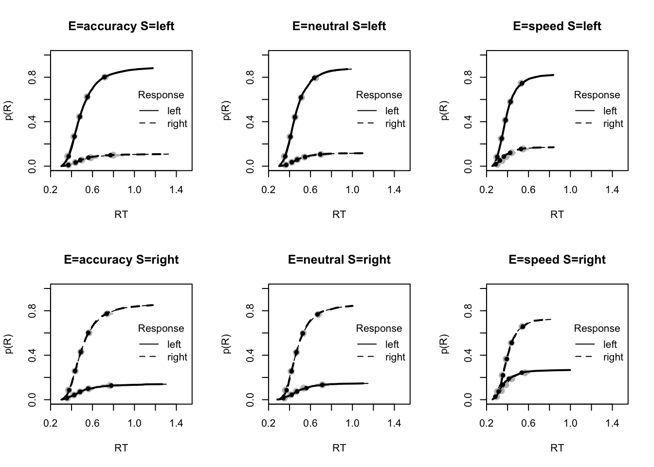
Now let’s look at the accuracy;
pc <- function(d) 100*mean(d$S==d$R)
# Excellent fit in all cases.
plot_fit(dat,ppPNAS_avt0_full,layout=c(2,3),factors=c("E","S"),
         stat=pc,stat_name="Accuracy (%)",xlim=c(70,95))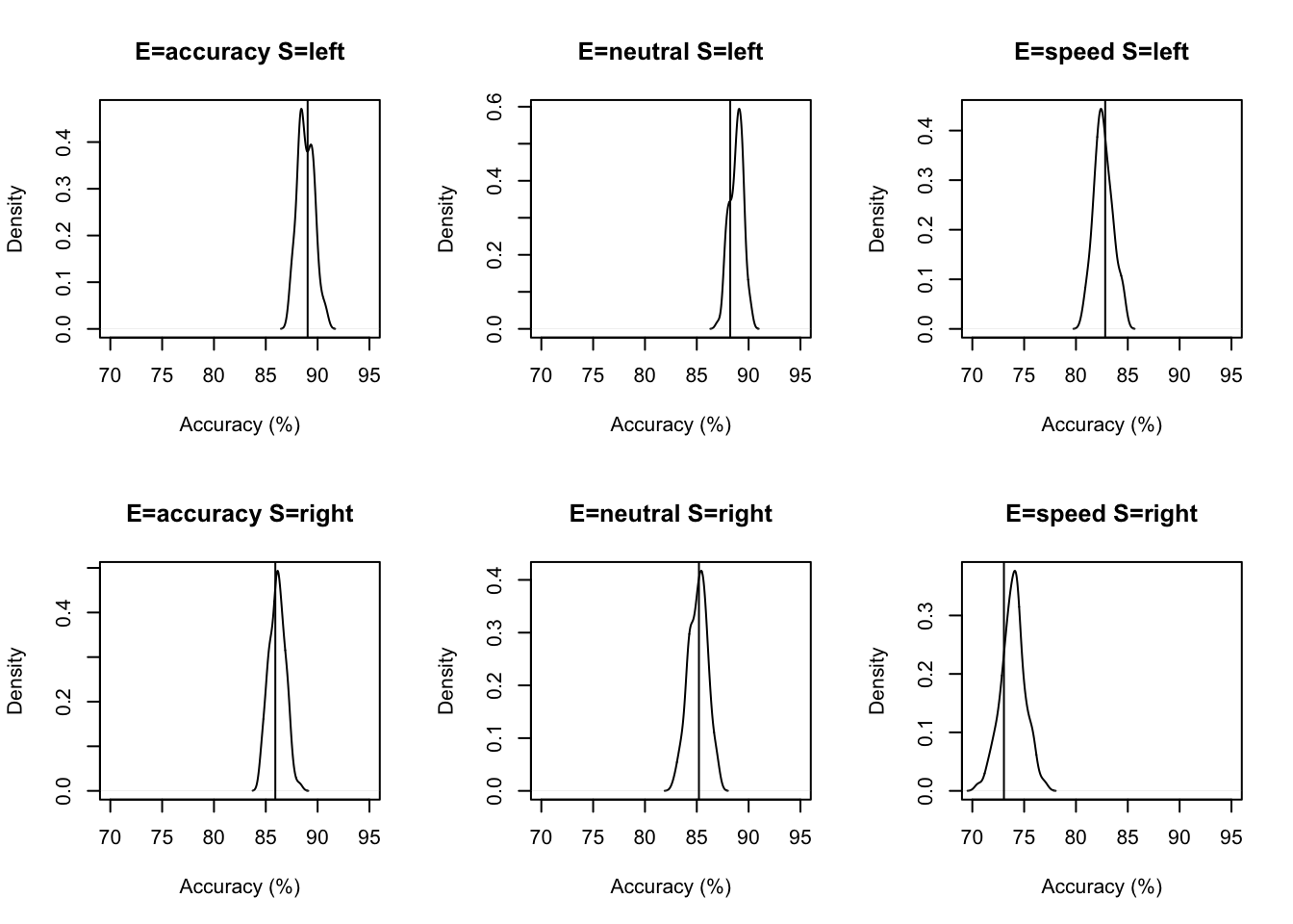
So far the full model appears to fit quite well. Let’s be clear though, the change here is not due to the cell coding, but rather due to us increasing the complexity of the model, so that more noise is captured by various parameters. For example, compared to the earlier models, including rates could be useful if there was an effect of stimulus and emphasis on the rates parameter, where people also concentrate more in the speed condition, leading to better accumulation of evidence. Let’s now look at some other pplots of fit;
# Mean RT also excellent
tab <- plot_fit(dat,ppPNAS_avt0_full,layout=c(2,3),factors=c("E","S"),
         stat=function(d){mean(d$rt)},stat_name="Mean RT (s)",xlim=c(0.375,.625))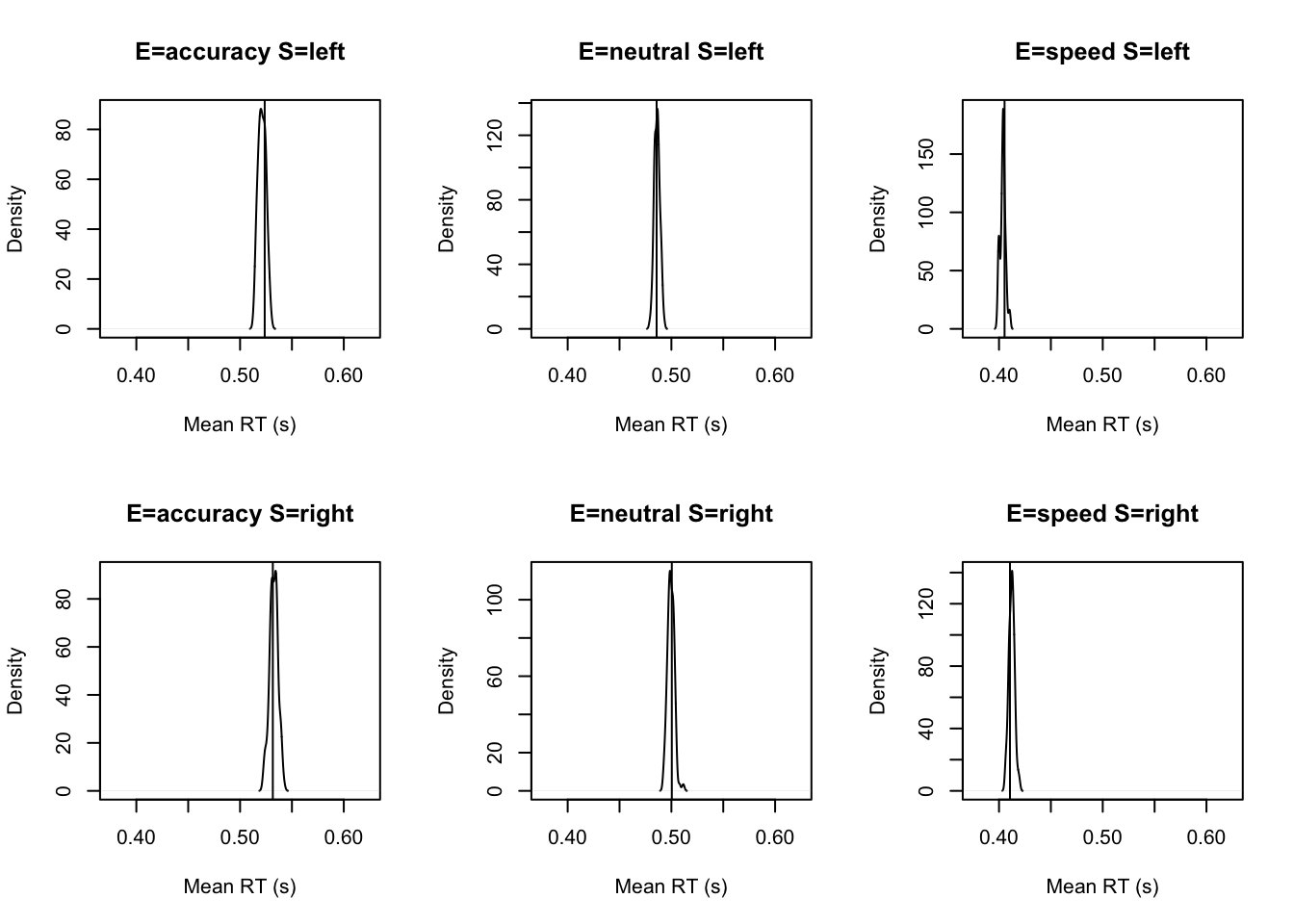
Response time fit is also excellent (however see below to look at some extreme quantile fits which are not as clean).
# However for fast responses (10th percentile) still some under-prediction except for speed.
tab <- plot_fit(dat,ppPNAS_avt0_full,layout=c(2,3),factors=c("E","S"),xlim=c(0.275,.375),
         stat=function(d){quantile(d$rt,.1)},stat_name="10th Percentile (s)")
round(tab,2)

# but for slow responses (90th percentile) all good.
tab <- plot_fit(dat,ppPNAS_avt0_full,layout=c(2,3),factors=c("E","S"),xlim=c(0.525,.975),
         stat=function(d){quantile(d$rt,.9)},stat_name="90th Percentile (s)")

# and RT variability now also good.
tab <- plot_fit(dat,ppPNAS_avt0_full,layout=c(2,3),factors=c("E","S"),
         stat=function(d){sd(d$rt)},stat_name="SD (s)",xlim=c(0.1,.355))


# Also errors speed also good, with some small residual over-estimation in speed.
tab <- plot_fit(dat,ppPNAS_avt0_full,layout=c(2,3),factors=c("E","S"),xlim=c(0.375,.725),
         stat=function(d){mean(d$rt[d$R!=d$S])},stat_name="Mean Error RT (s)")
round(tab,2)
Given we are confident that the model converged, everything went to plan with sampling and the fit looks good, we can now look at posterior parameter inference. Aagin, we won’t run these here, but we’ve left notes for you to try these out for yourself.
### Population mean (mu) tests

# Clearly the default N(0,1) priors are somewhat inappropriate for the large
# positive and negative rates produced by "cell" coding.
ciPNAS_avt0_full <- plot_density(sPNAS_avt0_full,layout=c(3,6),selection="mu",subfilter=500)

# Cell coding directly gives us the traditional drift rate estimates
round(ciPNAS_avt0_full,2)
## v_SEleft_accuracy v_SEright_accuracy v_SEleft_neutral v_SEright_neutral
## 2.5% -2.27 0.67 -2.44 0.60
## 50% -1.60 1.59 -1.73 1.57
## 97.5% -0.71 2.29 -0.79 2.30
## v_SEleft_speed v_SEright_speed a a_Eneutral a_Espeed sv t0
## 2.5% -2.19 -0.04 -0.12 -0.12 -0.46 -0.85 -1.38
## 50% -1.61 0.95 0.04 -0.09 -0.31 -0.35 -1.29
## 97.5% -0.81 1.70 0.19 -0.05 -0.11 0.06 -1.22
## t0_Eneutral t0_Espeed st0 Z SZ
## 2.5% -0.05 -0.23 -2.05 -0.14 -0.42
## 50% -0.01 -0.17 -1.89 -0.06 -0.14
## 97.5% 0.04 -0.12 -1.66 0.03 0.09# and (by definition) the same results when mapped
ciPNAS_avt0_full_mapped <- plot_density(sPNAS_avt0_full,layout=c(3,6),
selection="mu",mapped=TRUE,subfilter=500)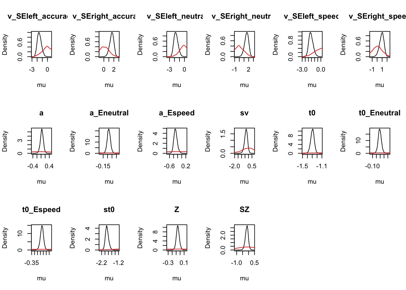
round(ciPNAS_avt0_full_mapped,2)## v_left_accuracy v_left_neutral v_left_speed v_right_accuracy v_right_neutral
## 2.5% -2.27 -2.44 -2.19 0.67 0.60
## 50% -1.60 -1.73 -1.61 1.59 1.57
## 97.5% -0.71 -0.79 -0.81 2.29 2.30
## v_right_speed a_accuracy a_neutral a_speed sv t0_accuracy t0_neutral
## 2.5% -0.04 0.89 0.82 0.66 0.43 0.25 0.25
## 50% 0.95 1.04 0.95 0.77 0.71 0.27 0.27
## 97.5% 1.70 1.21 1.10 0.91 1.06 0.29 0.29
## t0_speed st0 Z SZ
## 2.5% 0.21 0.13 0.45 0.34
## 50% 0.23 0.15 0.48 0.44
## 97.5% 0.25 0.19 0.51 0.54### t0 E effect
# Looking at the t0 effect of E there is no evidence of a accuracy-netural difference
p_test(x=sPNAS_avt0_full,x_name="t0_accuracy",y=sPNAS_avt0_full,y_name="t0_neutral",
subfilter=500,mapped=TRUE)## t0_accuracy t0_neutral t0_accuracy-t0_neutral
## 2.5% 0.25 0.25 -0.01
## 50% 0.27 0.27 0.00
## 97.5% 0.29 0.29 0.01
## attr(,"less")
## [1] 0.392# But speed is clearly less by ~40ms
p_test(x=sPNAS_avt0_full,subfilter=500,mapped=TRUE,x_name="t0: av(acc/neut)-speed",
x_fun=function(x){sum(x[c("t0_accuracy","t0_neutral")])/2 - x["t0_speed"]})## t0: av(acc/neut)-speed mu
## 2.5% 0.03 NA
## 50% 0.04 0
## 97.5% 0.06 NA
## attr(,"less")
## [1] 0# v E effect
# The pattern of E effects on rates suggests lower rates for speed, perhaps
# indicative of reduced selective attention and hence reduced discriminative
# quality of the evidence being processed.
fun <- function(x)
mean(abs(x[c("v_left_accuracy","v_left_neutral","v_right_accuracy",
"v_right_neutral")])) - mean(abs(x[c("v_left_speed","v_right_speed")]))
p_test(x=sPNAS_avt0_full,subfilter=500,mapped=TRUE,digits=3,
x_name="v: av(acc/neut)-speed",x_fun=fun)## v: av(acc/neut)-speed mu
## 2.5% 0.011 NA
## 50% 0.347 0
## 97.5% 0.633 NA
## attr(,"less")
## [1] 0.022# Although the effect is (barely) credible, one might also suspect over-fitting.
# In this case it would be useful to also fit models with selective influence of
# E on a and t0 vs. a and v. This is left as an exercise. 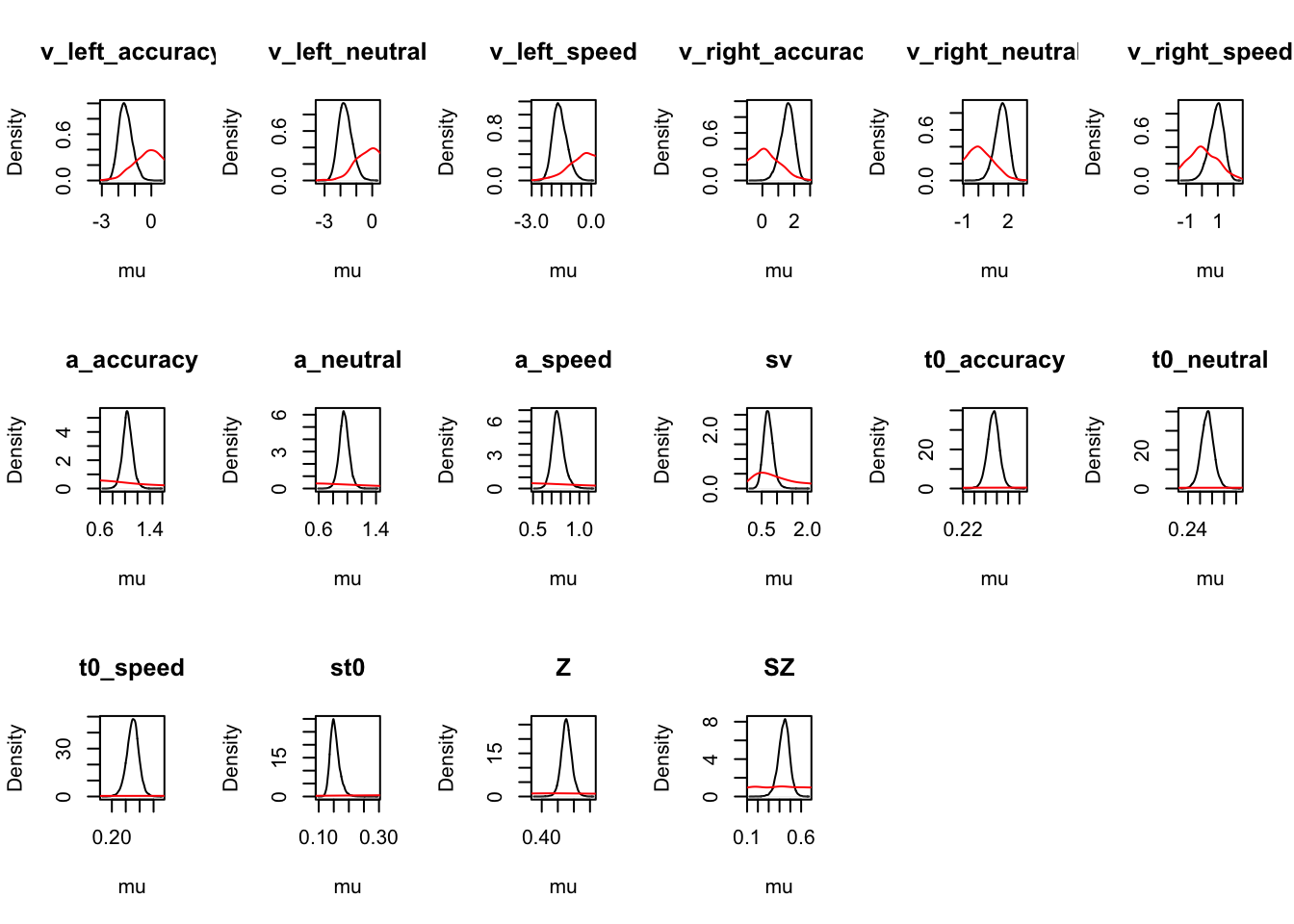
5.14 Model selection (briefly)
So far we’ve tested a few different models. These models vary in complexity, but also in quality of fit. So we may ask, “which model gives the best trade off between goodness of fit and simplicity?”. This is an important question for model-based sampling. So far we’ve looked at graphical metrics of fit, but these can be difficult to compare to one another. Information criteria (IC) approaches are commonly used to provide a single measure that describes the fit of the model, whilst attempting to account for complexity. These are based purely on the posterior samples. Here, we provide an IC function pmwg_IC that produces two types, DIC and BPIC (the latter gives greater weight to simplicity), where smaller values are better.
It also provides estimates of components of DIC and BPIC:
EffectiveN: the “effective” number of parameters (which is usually less than the actual number in hierarchical models)
meanD: the mean posterior deviance (which can also be used for model selection, but imposing only a weak complexity penalty)
Dmean: the deviance of the posterior parameter mean, which is a measure of goodness of fit
minD: an estimates of the minimum posterior deviance, the smaller of Dmean and the deviance for all samples (note that by default DIC and BPIC uses this value, base results on Dmean set use_best_fit=FALSE)
Let’s compare three of our models;
load("~/Desktop/emc2/models/DDM/DDM/examples/samples/sPNAS_a.RData")
load("~/Desktop/emc2/models/DDM/DDM/examples/samples/sPNAS_a_full.RData")
load("~/Desktop/emc2/models/DDM/DDM/examples/samples/sPNAS_avt0_full.RData")


pmwg_IC(sPNAS_a)
## DIC BPIC EffectiveN meanD Dmean minD
## -12957 -12828 129 -13086 728446 -13215pmwg_IC(sPNAS_a_full)## DIC BPIC EffectiveN meanD Dmean minD
## -16343 -16176 167 -16510 728446 -16677pmwg_IC(sPNAS_avt0_full,subfilter=500)## DIC BPIC EffectiveN meanD Dmean minD
## -17043 -16802 240 -17283 -17468 -17523pmwg_IC(sPNAS_a)## DIC BPIC EffectiveN meanD Dmean minD
## -12957 -12828 129 -13086 728446 -13215pmwg_IC(sPNAS_a_full)## DIC BPIC EffectiveN meanD Dmean minD
## -16343 -16176 167 -16510 728446 -16677pmwg_IC(sPNAS_avt0_full,subfilter=500)## DIC BPIC EffectiveN meanD Dmean minD
## -17043 -16802 240 -17283 -17468 -17523The nonsensical negative effective parameter count for the Wiener model is conventionally considered not to be a problem, but underlines that EffectiveN is best interpreted only in a relative sense. The other values are much more sensible and relative to the actual number of 19*10 = 190and 19*16=304 alpha parameters (random effects being relevant here as all of these calculations are based on the alpha posterior likelihoods), and are consistent with hierarchical shrinkage effects.
We see that the Wiener diffusion wins hugely in DIC/BPIC/meanD, despite its much worse goodness of fit in Dmean and Dmin (also evident in its strong qualitative failures shown graphically above). Overall this pattern suggests that the Wiener model be rejected.
The following function calculates model weights, quantities on the unit interval that under some further assumptions correspond to the probability of a model being the “true” model. Here clearly the avt0 model wins strongly.
compare_IC(list(avt0=sPNAS_avt0_full,a=sPNAS_a_full),subfilter=list(500,0))## DIC wDIC BPIC wBPIC EffectiveN meanD Dmean minD
## avt0 -17043 1 -16802 1 240 -17283 -17468 -17523
## a -16343 0 -16176 0 167 -16510 728446 -16677This is also true on a per-subject basis except for one participant.
compare_ICs(list(avt0=sPNAS_avt0_full,a=sPNAS_a_full),subfilter=list(0,500))## wDIC_avt0 wDIC_a wBPIC_avt0 wBPIC_a
## as1t 1.000 0.000 0.998 0.002
## bd6t 1.000 0.000 1.000 0.000
## bl1t 1.000 0.000 1.000 0.000
## hsft 1.000 0.000 1.000 0.000
## hsgt 0.433 0.567 0.139 0.861
## kd6t 1.000 0.000 1.000 0.000
## kd9t 1.000 0.000 1.000 0.000
## kh6t 1.000 0.000 1.000 0.000
## kmat 1.000 0.000 1.000 0.000
## ku4t 0.997 0.003 0.960 0.040
## na1t 0.999 0.001 0.994 0.006
## rmbt 1.000 0.000 0.999 0.001
## rt2t 1.000 0.000 1.000 0.000
## rt3t 1.000 0.000 1.000 0.000
## rt5t 1.000 0.000 1.000 0.000
## scat 0.998 0.002 0.990 0.010
## ta5t 1.000 0.000 1.000 0.000
## vf1t 1.000 0.000 1.000 0.000
## zk1t 1.000 0.000 1.000 0.000However, one might question whether we need both v and t0, so lets fit simpler models that drop one or the other.
design_at0_full <- make_design(
  Ffactors=list(subjects=levels(dat$subjects),S=levels(dat$S),E=levels(dat$E)),
  Rlevels=levels(dat$R),
  Flist=list(v~S,a~E,sv~1, t0~E, st0~1, s~1, Z~1, SZ~1, DP~1),
  constants=c(s=log(1),DP=qnorm(0.5)),
  model=ddmTZD)
## v v_Sright a a_Eneutral a_Espeed sv t0
## 0 0 0 0 0 0 0
## t0_Eneutral t0_Espeed st0 Z SZ
## 0 0 0 0 0
## attr(,"map")
## attr(,"map")$v
## v v_Sright
## 1 1 0
## 20 1 1
##
## attr(,"map")$a
## a a_Eneutral a_Espeed
## 1 1 0 0
## 39 1 1 0
## 77 1 0 1
##
## attr(,"map")$sv
## sv
## 1 1
##
## attr(,"map")$t0
## t0 t0_Eneutral t0_Espeed
## 1 1 0 0
## 39 1 1 0
## 77 1 0 1
##
## attr(,"map")$st0
## st0
## 1 1
##
## attr(,"map")$s
## s
## 1 1
##
## attr(,"map")$Z
## Z
## 1 1
##
## attr(,"map")$SZ
## SZ
## 1 1
##
## attr(,"map")$DP
## DP
## 1 1# samplers <- make_samplers(dat,design_at0_full,type="standard")
# save(samplers,file="sPNAS_at0_full.RData")
se <- function(d) {factor(paste(d$S,d$E,sep="_"),levels=
c("left_accuracy","right_accuracy","left_neutral","right_neutral","left_speed","right_speed"))}
design_av_full <- make_design(
Ffactors=list(subjects=levels(dat$subjects),S=levels(dat$S),E=levels(dat$E)),
Rlevels=levels(dat$R),
Clist=list(SE=diag(6)),
Flist=list(v~0+SE,a~E,sv~1, t0~1, st0~1, s~1, Z~1, SZ~1, DP~1),
Ffunctions = list(SE=se),
constants=c(s=log(1),DP=qnorm(0.5)),
model=ddmTZD)## v_SEleft_accuracy v_SEright_accuracy v_SEleft_neutral v_SEright_neutral
## 0 0 0 0
## v_SEleft_speed v_SEright_speed a a_Eneutral
## 0 0 0 0
## a_Espeed sv t0 st0
## 0 0 0 0
## Z SZ
## 0 0
## attr(,"map")
## attr(,"map")$v
## v_SEleft_accuracy v_SEright_accuracy v_SEleft_neutral v_SEright_neutral
## 1 1 0 0 0
## 39 0 0 1 0
## 77 0 0 0 0
## 20 0 1 0 0
## 58 0 0 0 1
## 96 0 0 0 0
## v_SEleft_speed v_SEright_speed
## 1 0 0
## 39 0 0
## 77 1 0
## 20 0 0
## 58 0 0
## 96 0 1
##
## attr(,"map")$a
## a a_Eneutral a_Espeed
## 1 1 0 0
## 39 1 1 0
## 77 1 0 1
##
## attr(,"map")$sv
## sv
## 1 1
##
## attr(,"map")$t0
## t0
## 1 1
##
## attr(,"map")$st0
## st0
## 1 1
##
## attr(,"map")$s
## s
## 1 1
##
## attr(,"map")$Z
## Z
## 1 1
##
## attr(,"map")$SZ
## SZ
## 1 1
##
## attr(,"map")$DP
## DP
## 1 1# samplers <- make_samplers(dat,design_av_full,type="standard")
# save(samplers,file="sPNAS_av_full.RData")
load("~/Desktop/emc2/models/DDM/DDM/examples/samples/sPNAS_avt0_full.RData")
load("~/Desktop/emc2/models/DDM/DDM/examples/samples/sPNAS_av_full.RData")
load("~/Desktop/emc2/models/DDM/DDM/examples/samples/sPNAS_at0_full.RData")
load("~/Desktop/emc2/models/DDM/DDM/examples/samples/sPNAS_a_full.RData")SZ was slow to converge in mu, needed to 750 for at0 and 500 for av, so ran enough samples to get 1000 left 1000 left without these.
All looks good with a_neutral now much more efficient
check_run(sPNAS_at0_full,subfilter=750)
check_run(sPNAS_av_full,subfilter=500,layout=c(3,5))
avt0 still wins overall
compare_IC(list(avt0=sPNAS_avt0_full,at0=sPNAS_at0_full,av=sPNAS_av_full,a=sPNAS_a_full),
            subfilter=list(500,750,500,0))
## DIC wDIC BPIC wBPIC EffectiveN meanD Dmean minD
## avt0 -17043 1 -16802 1 240 -17283 -17468 -17523
## at0 -16948 0 -16745 0 203 -17151 -17314 -17354
## av -16410 0 -16210 0 199 -16609 -16777 -16808
## a -16343 0 -16176 0 167 -16510 728446 -16677# But now there are 5 more equivocal cases, largely favoring the at0 model.
compare_ICs(list(avt0=sPNAS_avt0_full,at0=sPNAS_at0_full,av=sPNAS_av_full,a=sPNAS_a_full),
subfilter=list(500,750,500,0))## wDIC_avt0 wDIC_at0 wDIC_av wDIC_a wBPIC_avt0 wBPIC_at0 wBPIC_av wBPIC_a
## as1t 0.797 0.203 0.000 0.000 0.613 0.386 0.001 0.001
## bd6t 0.961 0.039 0.000 0.000 0.946 0.054 0.000 0.000
## bl1t 0.999 0.001 0.000 0.000 0.998 0.002 0.000 0.000
## hsft 0.992 0.008 0.000 0.000 0.985 0.015 0.000 0.000
## hsgt 0.330 0.271 0.101 0.298 0.170 0.173 0.056 0.602
## kd6t 0.436 0.564 0.000 0.000 0.205 0.795 0.000 0.000
## kd9t 0.606 0.394 0.000 0.000 0.303 0.697 0.000 0.000
## kh6t 0.834 0.166 0.000 0.000 0.706 0.294 0.000 0.000
## kmat 0.143 0.857 0.000 0.000 0.043 0.957 0.000 0.000
## ku4t 0.654 0.343 0.002 0.001 0.228 0.766 0.002 0.004
## na1t 0.039 0.961 0.000 0.000 0.013 0.987 0.000 0.000
## rmbt 0.989 0.010 0.001 0.000 0.973 0.017 0.010 0.001
## rt2t 0.998 0.002 0.000 0.000 0.987 0.013 0.000 0.000
## rt3t 0.926 0.074 0.000 0.000 0.780 0.220 0.000 0.000
## rt5t 1.000 0.000 0.000 0.000 0.999 0.000 0.001 0.000
## scat 0.075 0.925 0.000 0.000 0.024 0.976 0.000 0.000
## ta5t 0.997 0.003 0.000 0.000 0.998 0.002 0.000 0.000
## vf1t 0.991 0.009 0.000 0.000 0.958 0.042 0.000 0.000
## zk1t 0.911 0.089 0.000 0.000 0.776 0.224 0.000 0.000This is a classic method of testing and comparing models. However, IC methods can often be flawed. In the future sections, we show new, state of the art methods for model comparison, which accounts for the marginal likelihood of the model given the data.